Tag: Ham Radio

  • Step-by-step—Class 14

    Step-by-step—Class 14

    This is post 18 of 28 in the series “Amateur Radio”

    Posts about my adventures in amateur radio.

    1. Step by step – 1st Class
    2. Step-by-Step – 2nd Class
    3. Amateur Radio Codes of Conduct
    4. Step-by-Step – 3rd Class
    5. Step-by-Step – Class 4a
    6. Step-by-Step – Classes 4b & 4c
    7. Step-by-Step—Class 5
    8. Step-by-Step—Class 6
    9. Step-by-Step—Class 7
    10. Step-by-Step—Class 8a
    11. Step-by-Step—Class 8b
    12. Step-by-Step—Class 9
    13. Step-by-Step—Class 10
    14. Step-by-step—Class 11
    15. A Modern Code of Conduct and Ethics for Amateur Radio
    16. Step-by-step—Class 12
    17. Step-by-step—Class 13
    18. Step-by-step—Class 14
    19. Step-by-step—Class 15
    20. Step-by-step—Class 16
    21. Step-by-step—Class 17
    22. Reflection: My Amateur Radio Journey So Far
    23. Authorized to Transmit
    24. Starting the Next Chapter: Advanced & CW
    25. Making Winlink, Pat, ARDOP and a Yaesu FTdx10 Work on an Apple Silicon Mac
    26. Winlink on Apple Silicon: The Files, Scripts and One-Click Launcher
    27. Whispers around the world
    28. Week 2 of CW Class

    Tuning In: What I Learned About Radio Receivers from Al Penney’s Chapter 14

    A close-up view of a vintage Trio TS-530S HF transceiver showing its front panel controls and illuminated frequency display. The radio features numerous knobs and switches for functions such as load, plate, drive, band selection, AF and RF gain, mic gain, AGC, VOX, and meter settings. An analog meter on the left displays ALC and power readings, while a large central tuning knob dominates the lower middle of the panel. The equipment is part of a larger radio setup, with additional gear visible above and below the transceiver.
    A vintage Trio TS-530S HF transceiver. Image: John Parfrey.

    If you’ve been following my ham-radio learning journey, you already know that every week I come away from Al Penney’s RAC Basic class with at least one “aha!” moment. Chapter 14—Radio Receivers—was no exception. In fact, this one took me right back to 1985, when I was sitting at my test bench on the GFC Hammond shop floor with a scope probe in my hand, trying to figure out why a switching supply refused to behave.

    Receivers, it turns out, aren’t that different: they’re equal parts physics, architecture, and black-magic engineering. What follows are my notes and reflections on what Al covered—sensitivities, selectivities, superhets, noise sources, and that never-ending problem of intermod and cross-modulation that haunts every urban ham.

    What a Receiver Actually Has to Do

    I think most non-hams imagine a radio receiver as a kind of magical ear—just “listening” to signals floating around. In reality, it’s a chain of brutally practical engineering steps:

    1. Capture the RF using the antenna
    2. Select the one frequency we care about from thousands across the spectrum
    3. Amplify it without adding too much noise
    4. Recover the modulation—audio, data, or whatever information was riding on the carrier
    5. Amplify the audio and send it to a speaker, headphones, or computer interface

    Each block in that chain is an opportunity to either improve fidelity or seriously mess things up.

    This is why receiver performance is usually described by the “three Ss + D”: Sensitivity, Selectivity, Stability + Dynamic Range [1].

    Sensitivity: Hearing Signals That Barely Exist

    One of the wildest things about radio is just how small the signals are. At the antenna terminals, we’re often dealing with femtowatts—10-15 watts—yet after running through the receiver chain, we expect clean audio at the speaker.

    In modern HF rigs, sensitivity is rarely the limiting factor anymore. Al pointed out that, using SSB, the Kenwood TS-890 reliably hears down to 0.2 µV between 1.7 and 24.5 MHz [1]. That’s astonishing.

    But sensitivity ultimately runs into physics:

    Below ~30 MHz, the natural noise floor dominates.

    In other words, there’s no point trying to design an HF receiver with another 6 dB of sensitivity—galactic noise, atmospheric noise, and man-made noise swamp the front end long before the Low-Noise Amplifier (LNA) does.

    A few key measurements I found interesting:

    • Noise Figure (NF) – becomes critical at VHF/UHF where sky noise drops dramatically
    • MDS (Minimum Discernible Signal) – usually around −120 to −130 dBm for a good HF rig in 500 Hz BW
    • SNR and SINAD – important especially for FM receivers

    Signal-to-Noise And Distortion (SINAD):

    Where

    S = Signal

    N = Noise

    D = Distortion

    expressed in decibels (dB).

    Al Penney’s material notes:

    For a VHF or UHF receiver, SINAD is typically around 12 dB for an input of 0.25 µV (≈ −119 dBm).

    This is the standard sensitivity measurement used in commercial and amateur FM equipment.

    At VHF/UHF, the internal noise of that first transistor—your LNA—sets the limit. HF? Not so much.

    Selectivity: Where the Adults and Children Separate

    Selectivity is the receiver’s ability to separate two closely spaced signals. And this, more than raw sensitivity, is what earns premium radios their price tag.

    Al made a comment I loved:

    Filter skirt steepness is what separates the adults from the children in HF receiver design. [1]

    The skirts—the shape of the filter’s passband edges—determine how well a receiver rejects adjacent-channel interference. A typical SSB filter might have:

    • –6 dB bandwidth: ~2.3 kHz
    • –60 dB bandwidth: ~3.3 kHz

    A shape factor near 2:1 at 6/60 dB is excellent.

    A simple line graph showing the real frequency response of a band-pass filter. The central “Passband” region is relatively flat, while the response slopes downward on both sides into the “Stopband” areas. Vertical arrows mark the −6 dB points at the edges of the passband and the −60 dB points deeper into the stopband. The graph illustrates how an actual filter response deviates from an ideal rectangular shape, with rounded transitions and imperfect attenuation.
    Receiver Selectivity

    It’s worth appreciating just how much of our “receiver experience” is determined by these numbers. A crowded contest weekend on 20 m can turn a mediocre receiver into a miserable one.

    Digital Signal Processing (DSP) helps—adjustable bandwidth, notch filters, noise reduction—but the basic physics still matter.

    Stability: The End of Drifty Radios

    Anyone who has ever used an old tube rig on CW knows the pain of “chasing” your signal up or down the band as the oscillator warms up.

    Drift simply isn’t a major issue anymore. Modern PLL and DDS synthesizers with temperature-compensated oscillators typically achieve stability in the low parts-per-million (ppm) range [1].

    What DDS Does

    A DDS system creates RF signals digitally by:

    1. Using a numerically controlled oscillator (NCO)
    2. Stepping through a digital sine wave lookup table
    3. Converting the digital waveform to analog using a DAC (Digital-to-Analog Converter)
    4. Filtering the output to produce a clean RF signal

    This allows the radio’s VFO to tune in extremely fine steps (often <1 Hz) with excellent frequency stability.

    Why Radios Use DDS

    Compared with older analog VFOs or PLLs, DDS offers:

    • Very high frequency stability
    • Extremely fine tuning resolution
    • Fast frequency changes (great for scanning or DSP features)
    • Low drift, because it ultimately relies on a stable reference oscillator
    • Ability to implement complex waveforms (FSK, PSK, chirps)

    Still, your VFO is only as good as its reference. If the radio’s timebase drifts, so does every displayed frequency. That’s why Al reminded us to check against WWV, WWVH, or CHU periodically.

    Dynamic Range

    Although it doesn’t get listed alongside Sensitivity and Selectivity, the Dynamic Range of a receiver is every bit as important. It describes, in dB, the span of signal levels over which the radio can still do its job—pulling out the signals we actually care about without collapsing under the load. On the ham bands, this really matters because we routinely deal with whisper-weak signals sitting right beside blowtorch-strong ones, and a receiver with poor dynamic range simply can’t cope. There are a few different ways to measure it, but the rule of thumb is simple: the higher the dynamic range, the better the receiver will behave in real-world conditions.

    Cross-Modulation and Intermod: The Curse of Strong Signals

    Urban hams know this pain well: you’re trying to listen to a clean signal on 146.97 MHz, but the local taxi dispatcher or paging transmitter blasts into your receiver anyway.

    Two related but distinct demons cause this:

    Cross-modulation

    A strong AM signal overloads the front end, causing its modulation to appear on your desired signal. It shows up when:

    • You’re close to a high-power AM broadcast tower
    • Your front-end LNA is being driven into nonlinearity

    Attenuators help. So do front-end filters.

    Intermodulation (IMD)

    Two (or more) strong signals mix inside a nonlinear junction—an RF transistor, a mixer, even a rusty fence. This produces:

    • f1 ± f2
    • 2f₁ ± f₂
    • 2f2 ± f1, etc.

    On 2 m and 70 cm FM, IMD is especially brutal when driving through downtown due to the density of transmitters [1].

    A high third-order intercept point (IP3) is your best defence.

    A high IP3 is one of those specs that separates a decent receiver from a truly capable one. It’s a measure of how linear the receiver is—basically, how well it can deal with strong nearby signals without creating its own intermodulation junk. When multiple strong signals are floating around just outside your passband, a receiver with good IP3 will stay composed; a poor one will start generating intermod products that show up as false signals and make life miserable.

    The higher the IP3, the more signal the front end can tolerate before nonlinearities kick in and begin creating interference that wasn’t actually there. In real operating conditions—especially in busy urban RF environments or during contests—high IP3 performance is your best defence against overload, distortion, and those phantom signals that clutter up the band. It’s a key part of keeping the receiver clean, stable, and able to pull in the signal you actually care about.

    Explanation of Third-Order Intercept Point (IP3)

    • IP3 is a theoretical power level where the power of the third-order intermodulation products theoretically equals the power of the desired signal.
    • It defines the linearity limit of a receiver or amplifier; beyond this point, nonlinearities create distortion.
    • A higher IP3 indicates better linearity and less distortion at high signal levels, which are crucial for maintaining signal integrity in crowded or high-signal environments.

    Importance of high IP3 in Radio Receivers

    • Receivers with high IP3 are better at handling strong signals from nearby transmitters or multiple signals simultaneously without generating spurious signals.
    • This reduces false readings or signal interference, which is critical in applications such as amateur radio, communications, and radar.

    Noise, Noise Everywhere

    Noise sets the absolute bottom limit of what we can hear. Al divided it into two broad categories:

    Natural Noise (QRN)

    • Galactic background
    • Atmospheric static
    • Lightning

    Lightning bursts are wideband, energetic, and brutal—but noise blankers can help.

    Man-Made Noise (QRM)

    This is the stuff we fight all the time:

    • LED lightbulbs
    • Switching power supplies
    • Thermostats
    • EV chargers
    • Solar inverters
    • Grow lights (ask any ham living next to a basement gardener…)

    Al even mentioned Chinese HF radar systems—those rapid-fire pulses that light up the waterfall like a machine gun. We can’t fix those, but we can recognize them.

    The only real cure for local noise? Track it down and eliminate it at the source. A portable receiver is your best friend here.

    A Beautiful Example: The Humble Crystal Radio

    Al finished with a walk-through of the simplest possible receiver: the classic crystal set like the one I built as a kid. No power supply. No amplifier. Just:

    • A resonant LC circuit
    • A diode detector (originally galena with a cat-whisker)
    • High-impedance headphones
    Crystal radio wiring pictorial based on Figure 33 in Gernsback’s 1922 book “Radio For All” — JA.Davidson at the English Wikipedia, CC BY-SA 3.0, via Wikimedia Commons
    Crystal radio schematic. [4]

    The entire audio output is derived from the energy in the received RF signal. That still blows my mind—especially knowing how much we depend on active devices today.

    Crystal sets are a reminder that, at its core, radio is elegant physics. Everything else—DSP, PLL synthesizers, roofing filters—is refinement.

    Final Thoughts

    Every chapter in this course has filled gaps in my understanding, but this one tied everything together: noise, filters, amplifiers, mixers, all working in a carefully balanced dance. And as someone who spent a good chunk of the ’80s elbow-deep in analog circuits, it’s incredibly satisfying to revisit the fundamentals with fresh eyes.

    Next week, we move into transmitter architecture. I’m looking forward to it—and I’m already expecting another “aha!” moment.


    References

    [1] A. Penney, Radio Receivers (RAC Basic Course – Chapter 14), Radio Amateurs of Canada, 2025.

    [2] A. Z. Peebles, Communication System Principles, 4th ed. Reading, MA: Addison-Wesley, 1998.

    [3] American Radio Relay League (ARRL), The ARRL Handbook for Radio Communications, 100th ed. Newington, CT: ARRL, 2023.

    [4] B. Finio, ‘Build Your Own Crystal Radio’, Science Buddies. Accessed: Nov. 18, 2025. [Online]. Available: https://www.sciencebuddies.org/science-fair-projects/project-ideas/Elec_p014/electricity-electronics/crystal-radio

  • Step-by-step—Class 13

    Step-by-step—Class 13

    This is post 17 of 28 in the series “Amateur Radio”

    Posts about my adventures in amateur radio.

    1. Step by step – 1st Class
    2. Step-by-Step – 2nd Class
    3. Amateur Radio Codes of Conduct
    4. Step-by-Step – 3rd Class
    5. Step-by-Step – Class 4a
    6. Step-by-Step – Classes 4b & 4c
    7. Step-by-Step—Class 5
    8. Step-by-Step—Class 6
    9. Step-by-Step—Class 7
    10. Step-by-Step—Class 8a
    11. Step-by-Step—Class 8b
    12. Step-by-Step—Class 9
    13. Step-by-Step—Class 10
    14. Step-by-step—Class 11
    15. A Modern Code of Conduct and Ethics for Amateur Radio
    16. Step-by-step—Class 12
    17. Step-by-step—Class 13
    18. Step-by-step—Class 14
    19. Step-by-step—Class 15
    20. Step-by-step—Class 16
    21. Step-by-step—Class 17
    22. Reflection: My Amateur Radio Journey So Far
    23. Authorized to Transmit
    24. Starting the Next Chapter: Advanced & CW
    25. Making Winlink, Pat, ARDOP and a Yaesu FTdx10 Work on an Apple Silicon Mac
    26. Winlink on Apple Silicon: The Files, Scripts and One-Click Launcher
    27. Whispers around the world
    28. Week 2 of CW Class

    From Sparks to Sidebands: Learning Modulation All Over Again

    By Doug Nix, VE3— (future call sign pending!)

    When I started my electronics career at GFC Hammond Electronics in Guelph back in 1985, I spent my days testing and repairing linear and switch-mode power supplies. At the time, “modulation” meant watching ripple currents on the Tektronix scope or chasing a dead short upstream from an LM723 regulator. It wasn’t until I recently delved deeper into amateur radio that I began to appreciate how the same fundamental principles—mixing, switching, filtering, duty cycles, and harmonics—show up everywhere in RF.

    Last night’s RAC Basic lecture from Al Penney was another reminder that nearly every radio mode we use today is built on deceptively simple physical principles: change some characteristic of a carrier, and you can transport information across the planet. What changes is the cleverness with which we do it.

    This post is my attempt to capture what I learned, in my own words, with enough technical depth to keep it interesting.


    Continuous Wave (CW): Where Radio Began

    The earliest radio systems didn’t carry voice—they simply turned a carrier on and off. That’s continuous wave (CW), and it’s astonishingly robust, even in 2025.

    CW transmitter block diagram

    CW works because the information rate is slow and the bandwidth is tiny. That allows the receiver to use extremely narrow filters—sometimes only a few hundred hertz—which dramatically raises the signal-to-noise ratio. A CW signal can hide below the noise floor and still be copyable by a trained ear.

    Keyed sinusoidal waveform, like you might see from a CW transmitter

    One technical detail I found particularly interesting: the bandwidth of a keyed carrier is governed by the abruptness of the transitions. “Abruptness” refers to the slew rate of the switching waveform. More abrupt changes require a faster slew rate, which in turn creates harmonics. Slowing the corners on the waveform “softens” the transitions, thereby reducing or eliminating the harmonics.

    Hard keying produces broadband splatter due to the harmonics caused by the corners on the waveform—what old-timers call key clicks. So modern rigs shape those edges digitally to keep the spectrum clean.

    AM: The First Voice Mode—and the Inefficient One

    Amplitude Modulation was the first way we got voice on the air. It is also, by every modern measure, terribly inefficient.

    Why?

    Because an AM signal consists of:

    • A carrier (which carries no information)
    • A lower sideband
    • An upper sideband

    If your audio contains frequencies up to 6 kHz, the RF bandwidth becomes ±6 kHz on each side of the carrier—12 kHz total. Only the sidebands contain information; the carrier exists solely to help a simple diode demodulator recover the audio.

    This is why:

    • AM transmitters waste power on the carrier
    • AM takes up twice the necessary bandwidth
    • AM is inherently vulnerable to noise (almost all noise sources are amplitude-based)

    PEP (peak envelope power) becomes especially important in AM. A 100 W PEP transceiver can legally deliver only ~25 W of AM carrier because 100% modulation requires the envelope to swing to 4× the carrier power.

    Modulated waveform

    As someone who spent years debugging over-stressed power supplies, I now appreciate how much engineering went into keeping broadcast transmitters from exceeding that 100% limit. Overmodulation introduces phase reversals and spurious emissions extending theoretically to infinity—an EMC/Spectrum nightmare.

    Mixers: The Beating Heart of RF

    Al’s explanation of mixing echoed something I first learned at Hammond while troubleshooting transformers: non-linear systems create new frequencies.

    A mixer multiplies two signals:

    • Carrier frequency f1
    • Modulating or local oscillator frequency f2

    The output contains:

    • f1 + f2
    • f1 – f2
    • …plus other products if the device is imperfect, which it always is.

    This simple principle is what makes the superheterodyne receiver possible, and it’s how we shift an audio waveform up into the RF spectrum. Every mode—AM, FM, SSB, digital—depends on this idea.

    Sidebands and SSB: Why We Don’t Run AM Anymore

    In amplitude modulation, all the information is in the sidebands. Once you realize that both sidebands contain the same information, it becomes obvious: send only one.

    Enter Single Sideband (SSB)—a refinement of AM where:

    • One sideband is removed
    • The carrier is suppressed
    • Bandwidth is cut in half
    • Transmitted power is concentrated entirely in the useful spectrum

    That’s why SSB is the standard for HF voice. With a typical 3 kHz voice channel:

    • AM occupies ~6 kHz
    • SSB occupies ~2.7–3.0 kHz
    • FM occupies 10–15 kHz
    • And you can fit 2× as many SSB QSOs into a band as AM

    SSB also gives far better “punch” for the watt. A 100 W PEP SSB signal delivers voice peaks that punch through marginal conditions, and your average power is typically 10–20% of that unless you engage heavy speech processing [1].

    FM: Quieting, Capture, and Why VHF Sounds So Clean

    Frequency Modulation is a different animal. Instead of changing amplitude, we change the instantaneous frequency of the carrier.

    Two things make FM special:

    1. It rejects amplitude noise

    Because the information is in the frequency deviation, not amplitude, the receiver can use a limiter to discard all amplitude variation. That’s why FM broadcast radio sounds clean even with multipath, ignition noise, and urban interference.

    2. The Capture Effect

    If two FM signals are present on the same frequency, the stronger one “captures” the receiver. This is both a blessing (for repeaters) and a curse (for aviation, which uses AM, allowing overlapping transmissions to still be heard).

    FM also supports wideband (e.g., ±75 kHz for broadcast) and narrowband (typically ±2.5–5 kHz for amateur VHF/UHF).

    Carson’s Rule gives a quick estimate of FM bandwidth:

    BW ≈ 2 (Δf + fm)
    where Δf is peak deviation and fm is highest audio frequency.

    So a typical VHF ham radio:

    • ±3 kHz deviation
    • 3 kHz audio
    • BW ≈ 12 kHz

    No wonder we must be careful about over-deviating—your excitement literally widens your signal.

    Digital Modes: RTTY, Packet, and the March Toward Software

    Watching Al trace the evolution from Baudot, to AFSK, to modern sound-card decoding reminded me how far we’ve come from electromechanical teleprinters banging away in newsrooms.

    RTTY uses frequency shift keying (FSK):

    • One frequency = mark
    • Another = space
    • Typically ~170 Hz shift on HF

    Packet radio took the next step by wrapping data into structured frames with error detection (FCS) and acknowledgments—essentially, an early version of TCP/IP over RF.

    Today, software like fldigi, WSJT-X, and Direwolf replaces dozens of kilograms of mechanical equipment with a laptop and a USB cable.

    It’s astonishing to think that in my Hammond days, many of these digital modes were still hardware-based. Today, everything from modulation to filtering to demodulation is done numerically.

    Reflections as a New(er) Ham

    Studying modulation theory now—at this stage of my life—is a strange kind of homecoming. It’s refreshing, frankly. I’m reconnecting with the core physics and mathematics that first drew me into electronics before life led me into safety engineering, risk assessment, standards development, and consulting work.

    What strikes me most is that every mode is a tradeoff:

    • AM: simple but inefficient
    • SSB: efficient but harder to generate and tune
    • FM: noise-resistant but spectrally wide
    • CW: narrow and penetrating but slow
    • Digital: flexible but computationally heavy

    Each choice reflects a balance between bandwidth, power, complexity, and robustness—the same constraints I deal with every day in engineering safety systems.

    And that’s the joy of amateur radio: it’s the perfect intersection of physics, engineering, history, and pure hands-on experimentation.

    Can’t wait for the next chapter!


    References

    [1] A. Penney, Chapter 13 – Modulation and Transmitters. RAC Basic Qualification Course, Radio Amateurs of Canada. Ch13-Modulation-and-Transmitters

    [2] W. Sabin and E. Schoenike, HF Radio Systems & Circuits. New York, NY, USA: McGraw-Hill, 1998.

    [3] J. R. Carson, “Notes on the Theory of Modulation,” Proceedings of the IRE, vol. 10, no. 1, pp. 57–64, Feb. 1922.

    [4] E. H. Armstrong, “A Method of Reducing Disturbances in Radio Signaling by a System of Frequency Modulation,” U.S. Patent 1,941,066, filed Dec. 26, 1933, and issued Dec. 26, 1933.

    [5] Federal Communications Commission (FCC), Title 47 CFR Part 97 – Amateur Radio Service, U.S. Government Publishing Office, 2024.

    [6] A. B. Carlson, Communication Systems: An Introduction to Signals and Noise in Electrical Communication, 4th ed. New York, NY, USA: McGraw-Hill, 2002.

    [7] J. D. Kraus, Electromagnetics, 4th ed. New York, NY, USA: McGraw-Hill, 1992.

    [8] G. L. Tarkington and R. L. Ferrel, “The Single-Sideband Story,” QST, vol. 41, no. 7, pp. 17–23, July 1957.

    [9] M. Schwartz, W. R. Bennett, and S. Stein, Communication Systems and Techniques. New York, NY, USA: McGraw-Hill, 1966.

    [10] H. T. Friis and C. B. Feldman, “A Multiple-Unit Steerable Antenna for Short-Wave Radio Transmission,” Bell System Technical Journal, vol. 17, no. 2, pp. 337–364, Apr. 1938.

    [11] K. R. Hardis, “Understanding Peak Envelope Power,” QEX – Communications Quarterly, no. 169, pp. 3–10, Nov./Dec. 1995.

    [12] ITU Radiocommunication Bureau, ITU-R SM.328-12: Spectra and Bandwidth of Emissions, International Telecommunication Union, Geneva, 2015.

    [13] ITU Radiocommunication Bureau, ITU-R F.1110 – Frequency-Shift Keying and Keying Characteristics, International Telecommunication Union, Geneva, 2019.

    [14] L. E. Kahn, “Single-Sideband Transmission by Envelope Elimination and Restoration,” Proceedings of the IRE, vol. 40, no. 7, pp. 803–806, July 1952.

    [15] D. H. Johnson and J. E. Johnson, Modern Communications Systems: Principles and Applications. Boston, MA, USA: Pearson, 2010.

  • Step-by-step—Class 12

    Step-by-step—Class 12

    This is post 16 of 28 in the series “Amateur Radio”

    Posts about my adventures in amateur radio.

    1. Step by step – 1st Class
    2. Step-by-Step – 2nd Class
    3. Amateur Radio Codes of Conduct
    4. Step-by-Step – 3rd Class
    5. Step-by-Step – Class 4a
    6. Step-by-Step – Classes 4b & 4c
    7. Step-by-Step—Class 5
    8. Step-by-Step—Class 6
    9. Step-by-Step—Class 7
    10. Step-by-Step—Class 8a
    11. Step-by-Step—Class 8b
    12. Step-by-Step—Class 9
    13. Step-by-Step—Class 10
    14. Step-by-step—Class 11
    15. A Modern Code of Conduct and Ethics for Amateur Radio
    16. Step-by-step—Class 12
    17. Step-by-step—Class 13
    18. Step-by-step—Class 14
    19. Step-by-step—Class 15
    20. Step-by-step—Class 16
    21. Step-by-step—Class 17
    22. Reflection: My Amateur Radio Journey So Far
    23. Authorized to Transmit
    24. Starting the Next Chapter: Advanced & CW
    25. Making Winlink, Pat, ARDOP and a Yaesu FTdx10 Work on an Apple Silicon Mac
    26. Winlink on Apple Silicon: The Files, Scripts and One-Click Launcher
    27. Whispers around the world
    28. Week 2 of CW Class

    Getting on the Air: Lessons from Chapter 12 of the RAC Basic Certificate Course

    When you’re working toward your amateur radio certification, there’s a lot of theory to digest — regulations, electronics, antennas, propagation. But for most of us, the real excitement begins when we start to imagine what it’ll be like actually to get on the air. Al Penney’s Chapter 12 in the RAC Basic Certificate Course bridges that gap beautifully, showing how all the groundwork—resistors, Ohm’s law, decibels, and dBμV—comes together when you finally sit down at the radio, call sign in hand, and start operating for real. It’s a chapter that shifts the focus from knowing to doing.

    An AI generated image of a man sitting thoughtfully at a wooden desk in a warmly lit radio shack, wearing large headphones and tuning a vintage shortwave transceiver. The equipment glows with amber dials and meters, surrounded by switches, knobs, and a small keyboard. A world map hangs on the wall above the radio, alongside clocks and ham radio memorabilia. A desk lamp casts a focused light over the workspace, and a window reveals a soft daylight glow outside.

    From Q-Codes to Phonetics: Speaking the Language of Radio

    One of the earliest surprises for many new hams is just how structured on-air communication really is. Penney revisits the history of the Q-codes, developed around 1909 to help ships communicate across language barriers. Codes like QRP (“reduce power”) or QTH (“location”) remain in use today—succinct, efficient, and a reminder that brevity is part of good operating [1]. Having said that, Q-codes have been one of the big challenges for me. As a systems thinker, I look for internal logic in coding systems. Unfortunately, there isn’t an internal system for Q-codes, except at the highest level. Anyway, I’ll start with the most important ones, and if there are more that I need, I’m sure I’ll learn them as I need them 🤷‍♂️.

    Equally important is the phonetic alphabet, the backbone of clear voice communication. Whether you’re spelling out your call sign or confirming a grid locator, “Whiskey Delta Nine Tango Echo” is a lot clearer than “W-D-9-T-E” over a noisy channel. The modern NATO/ICAO phonetic alphabet, with words like Alfa, Bravo, and Juliett, dates to 1956 and remains standardized across aviation, maritime, and amateur services.

    NATO Phonetic Alphabet
    NATO/ICAO Phonetic Alphabet

    And then there are the many on-air abbreviations used when communicating by Morse Code on CW (just a few):

    • AR End of message
    • AS Wait
    • BK Break
    • BT Separator
    • K Over
    • KN Over (to specific station)
    • SK End of contact
    • etc.

    Then there’s HF, with SSB depending on the band and mode of communication, as well as digital modes such as Automatic Packet Reporting System (APRS), Amateur Teleprinting Over Radio (AMTOR), Phase Shift Keying, 31 Baud (PSK31), and others.

    It’s a lot. This is an elephant I need to eat a bite at a time.

    The Repeater: Your Gateway to the Airwaves

    For most beginners, the first contact happens through a repeater—that wonderful piece of infrastructure that listens on one frequency and simultaneously transmits your signal on another. These are full-duplex systems, often perched high on towers or mountain tops, dramatically extending your range beyond what a handheld or mobile rig could achieve on its own.

    Diagram showing how a radio repeater relays signals between two operators. On the left, Jim transmits on 146.16 MHz and receives on 146.76 MHz. On the right, Terry transmits on 146.16 MHz and receives on 146.76 MHz. A repeater positioned on a hill receives the lower frequency signal (146.16 MHz) and retransmits it on the higher frequency (146.76 MHz), allowing communication between the two operators who cannot directly hear each other.
    How communication with a radio repeater works

    Each repeater pair operates with a standard offset—typically 600 kHz on the 2 m band—and may require a PL (CTCSS) tone to access. If your local machine needs a 136.5 Hz tone and you forget to program it, you’ll be talking to yourself! These tones prevent repeaters from keying up in response to stray interference and are crucial in maintaining a civil and usable spectrum.

    On the Air: First QSOs and Good Etiquette

    Penney devotes an entire section to that moment every new ham remembers—the first QSO. The key takeaway? Listen first. Nothing will endear you faster to your local club than showing patience and situational awareness before you key up. Once you do, identify clearly, use your call sign at the start and end of each contact, and every 30 minutes in between. Never “kerchunk” the repeater (key up without identifying) just to test your signal—that’s poor form and, technically, illegal.

    Al’s guidance on etiquette reads like a master class in radio citizenship. Give others a chance to use the repeater, keep conversations courteous and on-topic, and remember that repeaters are shared resources. Even small gestures—like helping maintain the repeater site or simply donating a few dollars to the local club—go a long way toward keeping our networks alive.

    HF Operating: Beyond the Repeater

    If VHF and UHF are your local playgrounds, HF is where you discover the world. Penney’s treatment of HF operation in this chapter demystifies what can seem like chaos: no channels, variable signal strength, fading (QSB), and the ever-present QRN of static. The key difference is that HF communication relies on the ionosphere, where refraction allows signals to bend around the globe—but also fade, flutter, and overlap in unpredictable ways.

    SSB operation (upper sideband above 30 m, lower sideband below) dominates HF phone communication for its bandwidth efficiency—roughly 3 kHz compared to FM’s 15–20 kHz. Combine that with proper filtering, good receiver selectivity, and a healthy dose of patience, and suddenly you’re working stations thousands of kilometres away with only a hundred watts and a length of wire in the trees.

    The Spirit of Amateur Radio

    Perhaps the most valuable insight from this chapter isn’t technical at all—it’s cultural. Whether through repeaters, satellites, or CW on a quiet 40-meter band, amateur radio is as much about how we operate as it is about what we operate. Penney closes with a reminder that respect, curiosity, and generosity are the invisible glue that keeps this community together. Every “73” sent across the airwaves carries a little of that tradition forward.


    References

    [1] A. Penney, RAC Basic Certificate Course: Chapter 12 – Operating a Station, Radio Amateurs of Canada, 2024.
    [2] “NATO Phonetic Alphabet,” Wikipedia, https://en.wikipedia.org/wiki/NATO_phonetic_alphabet.
    [3] “IRLP and EchoLink,” Amateur Radio Wiki, 2023.
    [4] “Ham Radio 101: Digital Signal Processing,” HamRadioSchool.com, 2023.

  • A Modern Code of Conduct and Ethics for Amateur Radio

    A Modern Code of Conduct and Ethics for Amateur Radio

    This is post 15 of 28 in the series “Amateur Radio”

    Posts about my adventures in amateur radio.

    1. Step by step – 1st Class
    2. Step-by-Step – 2nd Class
    3. Amateur Radio Codes of Conduct
    4. Step-by-Step – 3rd Class
    5. Step-by-Step – Class 4a
    6. Step-by-Step – Classes 4b & 4c
    7. Step-by-Step—Class 5
    8. Step-by-Step—Class 6
    9. Step-by-Step—Class 7
    10. Step-by-Step—Class 8a
    11. Step-by-Step—Class 8b
    12. Step-by-Step—Class 9
    13. Step-by-Step—Class 10
    14. Step-by-step—Class 11
    15. A Modern Code of Conduct and Ethics for Amateur Radio
    16. Step-by-step—Class 12
    17. Step-by-step—Class 13
    18. Step-by-step—Class 14
    19. Step-by-step—Class 15
    20. Step-by-step—Class 16
    21. Step-by-step—Class 17
    22. Reflection: My Amateur Radio Journey So Far
    23. Authorized to Transmit
    24. Starting the Next Chapter: Advanced & CW
    25. Making Winlink, Pat, ARDOP and a Yaesu FTdx10 Work on an Apple Silicon Mac
    26. Winlink on Apple Silicon: The Files, Scripts and One-Click Launcher
    27. Whispers around the world
    28. Week 2 of CW Class

    Code of Conduct and Ethics for Amateur Radio Operators

    Preamble

    Amateur radio is more than a hobby—it is a global community built on curiosity, respect, and public service. Every licensed operator shares responsibility for preserving the integrity and spirit of amateur radio. This Code establishes the ethical foundation for operating practice, personal conduct, and service to others within the amateur radio community.


    1. Core Principles

    1.1 Considerate

    An amateur radio operator acts courteously and never knowingly interferes with the communications or enjoyment of others. Respect for shared spectrum is the foundation of good operating practice.

    1.2 Responsible

    The responsible operator:

    • Complies fully with national and international regulations.
    • Uses equipment and techniques that meet accepted technical standards.
    • Exercises restraint and good judgment in all transmissions.

    1.3 Progressive

    The progressive operator:

    • Strives to improve technical knowledge, station performance, and operating skill.
    • Embraces new technologies and methods while preserving the traditions that sustain amateur radio.
    • Shares experience and promotes continuous learning.

    1.4 Helpful

    The helpful operator:

    • Offers assistance, support, and encouragement to others, especially newcomers.
    • Freely shares knowledge, promotes safety, and fosters self-reliance.
    • Helps maintain a cooperative and educational atmosphere on the air.

    1.5 Friendly

    The friendly operator:

    • Demonstrates patience and understanding.
    • Communicates with warmth and good humour.
    • Builds goodwill across boundaries of geography, language, and culture.

    1.6 Tolerant

    The tolerant operator:

    • Recognizes that others may hold different opinions or operating styles.
    • Responds to disagreement or interference calmly, without hostility or insult.
    • Practices empathy and inclusion in every interaction.

    1.7 Balanced

    The balanced operator:

    • Keeps amateur radio in proper perspective among personal, family, professional, and community responsibilities.
    • Recognizes that radio is a hobby and not a substitute for real-world obligations.

    1.8 Loyal

    The loyal operator:

    • Supports the amateur community, local clubs, and national societies that represent amateur radio interests regionally and internationally.
    • Acts to strengthen cooperation within the International Amateur Radio Union (IARU) community.

    1.9 Public-Spirited

    The public-spirited operator:

    • Offers knowledge, equipment, and skill in the service of community, public safety, and humanitarian needs.
    • Supports emergency and disaster communication whenever possible.
    • Acts with integrity and neutrality in public service roles.

    1.10 Ethical

    The ethical operator:

    • Conducts all activities with honesty, fairness, and respect for others.
    • Never deliberately transmits false information, causes harmful interference, or acts maliciously.
    • Upholds the self-discipline and integrity that define the amateur radio tradition.

    2. Guiding Values

    1. Respect: Every contact—on the air or in person—should demonstrate courtesy and mutual regard.
    2. Politeness: Language and tone should reflect self-control and dignity; abusive or inflammatory speech has no place in amateur radio.
    3. Self-discipline: Amateur radio is self-policing; each operator bears responsibility for maintaining order and goodwill on the bands.
    4. Learning and mentorship: Share your knowledge, teach others, and welcome newcomers to the hobby.
    5. Accountability: Recognize that your actions on the air reflect on all amateur radio operators.
    6. Integrity in competition: Pursue operating awards and contests fairly and honestly; never falsify logs or use deception.
    7. Environmental and safety awareness: Operate with respect for neighbours, communities, and the environment.

    3. Commitment to the Amateur Spirit

    The amateur spirit embodies cooperation, curiosity, and service. It transcends nationality, language, and generation. To honour that spirit, each operator pledges to:

    • Uphold the highest standards of conduct and ethics on the air and online.
    • Serve as a positive example to others.
    • Promote international friendship and understanding through radio communication.
    • Continue learning, experimenting, and contributing to the advancement of radio art.

    4. Closing Statement

    This Code is not a set of rules to restrict enjoyment but a framework that protects it. By following these principles, every amateur ensures that the bands remain a place of learning, goodwill, and public service for future generations.


    Adapted and unified from:

    • The Radio Amateur’s Code (Paul M. Segal, W9EEA, 1928)
    • Code of Ethics for Canadian Amateur Radio Operators (Bill Wilson, VE3NR)
    • Ethics and Operating Procedures for the Radio Amateur, ITU Endorsed, 2010 Ethics and operating Procedures…

    Download a copy

  • Step-by-Step—Class 10

    Step-by-Step—Class 10

    This is post 13 of 28 in the series “Amateur Radio”

    Posts about my adventures in amateur radio.

    1. Step by step – 1st Class
    2. Step-by-Step – 2nd Class
    3. Amateur Radio Codes of Conduct
    4. Step-by-Step – 3rd Class
    5. Step-by-Step – Class 4a
    6. Step-by-Step – Classes 4b & 4c
    7. Step-by-Step—Class 5
    8. Step-by-Step—Class 6
    9. Step-by-Step—Class 7
    10. Step-by-Step—Class 8a
    11. Step-by-Step—Class 8b
    12. Step-by-Step—Class 9
    13. Step-by-Step—Class 10
    14. Step-by-step—Class 11
    15. A Modern Code of Conduct and Ethics for Amateur Radio
    16. Step-by-step—Class 12
    17. Step-by-step—Class 13
    18. Step-by-step—Class 14
    19. Step-by-step—Class 15
    20. Step-by-step—Class 16
    21. Step-by-step—Class 17
    22. Reflection: My Amateur Radio Journey So Far
    23. Authorized to Transmit
    24. Starting the Next Chapter: Advanced & CW
    25. Making Winlink, Pat, ARDOP and a Yaesu FTdx10 Work on an Apple Silicon Mac
    26. Winlink on Apple Silicon: The Files, Scripts and One-Click Launcher
    27. Whispers around the world
    28. Week 2 of CW Class
    My Hammond Manufacturing business card from 1989.
    My business card at GFC prior to the spin-off of the organization in 1989

    From Hammond to High Efficiency: Reflections on Power Supplies Then and Now

    In 1985, when I started my career at GFC Hammond Electronics in Guelph, Ontario, the hum of transformers and the scent of flux were part of my daily environment. As a production test technician, my job was to test and repair linear and switching power supplies—work that gave me an intuitive feel for what really makes electronic systems tick.

    Four men kneel in front of a sign reading “Hammond Manufacturing Company Limited” with divisions listed as “GFC/Hammond Electronics Division,” “Hammond Electronics Division,” and “Hammond Museum of Radio.” The sign is mounted outside an industrial building with white and dark metal siding. Two of the men wear light blue lab coats, and the group poses on a grassy area under a clear blue sky.
    1989 – L-R: Bruce Ritchie (QA Manager), me, a Korean colleague, and Jerry Williamson (Manufacturing Engineering) in front of the Curtis Road plant in 1989.

    The Hammond facility on Curtis Road was a fascinating place for someone just starting out in electronics. The Hammond Museum of Radio was located in the same building, and the local amateur radio club’s repeater, VE3HC, had a tower at the back of the plant. Fred Hammond himself—whose name is etched into Canadian radio history—could often be found tinkering or chatting with staff. For a young technician like me, those were inspiring encounters that linked the practical side of my work to a century of radio innovation.

    Understanding the Foundations

    To appreciate modern power supplies, it helps to look back to the origins of the electrical grid itself. The way we generate and distribute electricity has always shaped the way we convert it.

    In the late 19th century, the “War of the Currents” pitted two of the era’s greatest inventors against each other: Thomas Edison, who favoured direct current (DC), and Nikola Tesla, whose alternating current (AC) system was backed by George Westinghouse. Edison’s DC approach had the advantage of simplicity and safety, but it couldn’t transmit power efficiently over long distances. Tesla’s AC system, on the other hand, used transformers to step voltage up for transmission and down for use—making large-scale distribution practical for the first time.

    The debate was settled decisively in 1895, when the Niagara Falls hydroelectric plant—built by Westinghouse—demonstrated the superiority of AC power. The plant’s generators produced 25 Hz alternating current, a frequency chosen as a compromise between efficient motor operation and adequate lighting performance. While 25 Hz served early heavy industry well, it wasn’t ideal for all applications. By the early 20th century, 60 Hz had become North America’s standard, striking a balance between efficiency and performance for the emerging electrical grid. [2]

    Across the Atlantic, Europe standardized on 50 Hz, largely through the influence of engineers at AEG and the VDE. They determined that 50 Hz offered the best trade-off between voltage drop, lighting flicker, and motor design. The choice was also elegantly compatible with the metric system—a detail the Germans took no small satisfaction in noting. [1]

    These early engineering decisions still echo in our wall sockets today. The world’s grids may differ by frequency and voltage, but they all deliver alternating current—a form of power distribution optimized for transmission, not for the needs of modern electronics.

    Why Electronics Need Conversion

    For electronic systems, line-frequency AC power isn’t directly useful. Radios, computers, and control circuits all require direct current (DC)—and not just any DC, but clean, stable, and precisely regulated voltage. This is where power converters come in: they transform AC into DC and sometimes back into AC at different frequencies for specialized uses, such as motor drives or RF systems.

    This need for efficient and reliable power conversion drives the evolution from linear to switch-mode power supplies—the very technologies I worked on daily at Hammond.

    Linear Power Supplies

    In a traditional linear power supply, the transformer does the heavy lifting, stepping up or down the voltage and isolating the circuit from the mains. The rectifier converts AC to DC—first through simple half- or full-wave circuits and later through the now-ubiquitous bridge rectifier. The resulting pulsating DC is smoothed by large electrolytic capacitors, which store charge between cycles to reduce ripple.

    Filtering and regulation define the character of a linear supply. Early designs used Zener diodes or discrete transistor regulators, which three-terminal IC regulators, such as the LM78xx series later replaced. Linear regulators operate in the transistor’s linear region, dropping excess voltage as heat—a simple, reliable, and noisy (in the thermal sense) way to achieve a stable output.

    Linear supplies have an unmistakable presence: heavy transformers, warm chassis, and that faint 120-Hz hum that signalled a tired filter capacitor. They were dependable, repairable, and forgiving—a good match for the analog age.

    Schematic diagram of a vacuum tube power supply circuit using a Hammond 270FX transformer and a 5U4GB rectifier tube. The primary side is connected to AC mains with a fuse and power switch. The secondary has a 275-0-275 V winding feeding the 5U4GB full-wave rectifier, along with 5 V and 6.3 V heater windings. The rectified DC passes through a multi-stage LC filter composed of Hammond 193J (10 H, 82 Ω) and Hammond 158Q (5 H, 150 Ω) chokes, plus 32 µF and 100 µF filter capacitors. A 350 Ω 5 W resistor provides additional filtering, and a 470 kΩ bleeder resistor is connected to ground. The output B+ voltage is approximately 272 V DC.
    A Vacuum tube rectified DC power supply for a tube amplifier. The B+ voltage has the same function as Vcc in semiconductor circuits.

    Because linear supplies operate in the linear region of the transistors, the difference between the raw rectified DC and the output voltage must be dropped across the regulator transistor(s), resulting in significant I2R losses in those devices. [4], [5].

    Schematic diagram of a regulated DC power supply using a full-wave bridge rectifier and an LM7805 voltage regulator. AC voltage from a transformer secondary is fed into a bridge rectifier made up of four diodes (D1–D4) arranged in a diamond pattern. The rectified output is filtered by capacitors C1 and C2, then passed through an LM7805 regulator that outputs a stable +5 V DC. A final smoothing capacitor C3 is connected at the output.
    Linear 5 Vdc regulated power supply. The rating of the LM7805 regulator limits the output current from this design. [4]

    From Linear to Switching

    By the time I arrived at Hammond, switch-mode power supplies (SMPS) were reshaping the field. Instead of relying on bulky transformers at 60 Hz, SMPS designs rectify the AC first, then chop the DC at high frequency—tens or hundreds of kilohertz—using transistors operating in saturation (fully on or off). The high frequency allows much smaller transformers and capacitors, dramatically improving efficiency and reducing weight.

    Of course, early SMPS units had their quirks. Without proper filtering—MOVs, chokes, and capacitors on the input—they could fill an HF receiver’s spectrum with a wash of interference. However, as designs matured, improved EMI filters, shielding, and power factor correction made switching supplies both quieter and more efficient.

    How switching power supplies work

    In switch-mode supplies, the AC mains power is first rectified. Then, the DC power is converted back to AC at a much higher frequency, allowing smaller, lighter, and less expensive transformers to be used to provide the lower AC voltages needed for the load(s). The use of higher frequencies also means that the filter capacitors can be smaller in size and lighter in weight. Additional inductors are required to prevent high-frequency switching noise from transferring to the load side of the supply. The benefit is that the primary power converter can use pulse-width modulation, keeping the switching transistors operating in their saturation mode, and thereby reducing the I2R losses in the transistors that result in waste heat. [6], [7].

    Circuit diagram of a TL594-based switch mode power supply (SMPS) with battery over- and under-voltage protection, designed by Gary Lecomte. The TL594 PWM controller IC drives two MOSFETs (IRF640 or STP75NF75) connected in a push-pull configuration to a ferrite core transformer (T1). The primary side operates from a 12 V DC input, filtered by a 220 µF capacitor. Frequency control is set by resistors Ra (8.2 kΩ), Rb (10 kΩ), and capacitor C1 (0.0022 µF), producing a switching frequency between 35 kHz and 70 kHz depending on adjustment. A 2N3904 transistor provides voltage error feedback for regulation. The secondary winding of the transformer is rectified by a diode bridge to produce a DC output. The circuit includes overvoltage protection at about 15.5 V and undervoltage protection at about 11 V, with additional notes explaining frequency and dead-time adjustment.

    What’s easy to forget is that early SMPS units were not always well-behaved neighbours in a radio shack. Without proper transient filtering—MOVs, chokes, and capacitors on the input—they could turn the HF spectrum into a wash of hash. Today’s designs, with improved EMI filtering and power factor correction, are worlds better.

    Lessons That Endure

    Looking back, my time at Hammond laid a foundation for everything that followed. Power supplies are not just supporting components; they’re the heart of every electronic system. If the supply isn’t clean, stable, and appropriately rated, nothing downstream behaves as intended.

    Al Penney’s excellent presentation [3] on power supplies for amateur radio operators captures that same truth: whether you’re winding transformers, testing LM7805 regulators, or designing 90%-efficient SMPS circuits, the goal remains constant—reliable, safe power delivery.

    For me, that journey began on a test bench in Guelph, soldering iron in one hand and scope probe in the other—under the same roof where Fred Hammond preserved the history of radio. It’s a fitting reminder that every modern innovation, no matter how advanced, still rests on a well-built power supply.


    References

    [1] G. Neidhöfer, ‘50-Hz Frequency [History]’, IEEE Power and Energy Mag., vol. 9, no. 4, pp. 66–81, July 2011, doi: 10.1109/MPE.2011.941165.

    [2] P. Mixon, ‘Technical origins of 60 Hz as the standard AC frequency in North America’, IEEE Power Eng. Rev., vol. 19, no. 3, pp. 35–37, Mar. 1999, doi: 10.1109/MPER.1999.1036103.

    [3] A. Penney, Power Supplies, VO1NO, RAC Basic Amateur Radio Course, 2023.

    [4] O. M. Urias, ‘How to Build a DC Linear Power Supply’, Build Electronic Circuits. Accessed: Oct. 30, 2025. [Online]. Available: https://www.build-electronic-circuits.com/linear-power-supply/

    [5] ‘Power Supply Circuits’, in Lessons in Electric Circuits. Accessed: Oct. 29, 2025. [Online]. Available: https://www.allaboutcircuits.com/textbook/semiconductors/chpt-9/power-supply-circuits/

    [6] “Switching Mode Power Supplies,” Wikipedia. [Online]. Available: https://en.wikipedia.org/wiki/Switched-mode_power_supply

    [7] C. Atwell, ‘A Brief History of Switching Power Supplies’, Electronic Design. Accessed: Nov. 07, 2025. [Online]. Available: https://www.electronicdesign.com/technologies/power/article/55040799/electronic-design-switching-power-supply-history-from-theory-to-design-essential

  • Step-by-step—Class 11

    Step-by-step—Class 11

    This is post 14 of 28 in the series “Amateur Radio”

    Posts about my adventures in amateur radio.

    1. Step by step – 1st Class
    2. Step-by-Step – 2nd Class
    3. Amateur Radio Codes of Conduct
    4. Step-by-Step – 3rd Class
    5. Step-by-Step – Class 4a
    6. Step-by-Step – Classes 4b & 4c
    7. Step-by-Step—Class 5
    8. Step-by-Step—Class 6
    9. Step-by-Step—Class 7
    10. Step-by-Step—Class 8a
    11. Step-by-Step—Class 8b
    12. Step-by-Step—Class 9
    13. Step-by-Step—Class 10
    14. Step-by-step—Class 11
    15. A Modern Code of Conduct and Ethics for Amateur Radio
    16. Step-by-step—Class 12
    17. Step-by-step—Class 13
    18. Step-by-step—Class 14
    19. Step-by-step—Class 15
    20. Step-by-step—Class 16
    21. Step-by-step—Class 17
    22. Reflection: My Amateur Radio Journey So Far
    23. Authorized to Transmit
    24. Starting the Next Chapter: Advanced & CW
    25. Making Winlink, Pat, ARDOP and a Yaesu FTdx10 Work on an Apple Silicon Mac
    26. Winlink on Apple Silicon: The Files, Scripts and One-Click Launcher
    27. Whispers around the world
    28. Week 2 of CW Class

    Building the Heart of the Shack

    When I was starting out in electronics in the mid-1980s, the idea of having a well-equipped radio shack had a kind of magic to it (it still does!).

    Not my shack, but it sure looks nice!

    At GFC Hammond in Guelph, where I first worked as a production test technician, I’d wander through the Hammond Museum of Radio on my lunch breaks, looking at the early receivers and transmitters that once connected Canada to the world. Those glass-tubed wonders seemed impossibly far from my world of circuit boards and switching supplies—but they planted the seed.

    Now, after years of working with safety systems, standards, and industrial controls, I find the simplicity of amateur radio refreshing. It’s a space where you can still build something tangible—wire, solder, and ingenuity turning into a working station that reaches across continents.

    Choosing the Right Space

    Al Penny starts Chapter 11 of the RAC course with a point that sounds simple but matters immensely: location is everything. Whether your shack is in the basement, a spare room, or tucked into a corner of your office, comfort, safety, and practicality all count. I’ve seen too many setups crammed into damp basements where corrosion becomes a silent saboteur. On the flip side, attic shacks turn into saunas by July. [1]

    The key is access—to power, grounding, and a clean route for feed lines and rotator cables. The rest—furniture, décor, and clever cable management—comes later. What matters most is making a space you actually want to spend time in. After all, this is where you’ll chase DX at 2 a.m., rebuild an antenna tuner that “worked fine yesterday,” and tinker endlessly with wiring diagrams.

    The Gear: New, Used, and Everything in Between

    Penny gives solid advice on buying equipment: define your needs first, then go shopping. The market today is overflowing with excellent radios, from handhelds that fit in a jacket pocket to sophisticated HF rigs that rival commercial equipment. The temptation to overspend is real.

    Buying used gear can be a fantastic way to stretch your budget—but it’s a bit like dating. You need to know what you’re getting into. Check for drift, dirty switches, and tell-tale signs of neglect. A radio that looks like it’s been through a sandstorm probably has. But when you find the right piece—an older Icom or Kenwood that’s been well-loved and well-maintained—it can serve faithfully for years.

    Whether you buy new or used, read the reviews, talk to other hams, and don’t underestimate the value of a dealer warranty. Sometimes peace of mind is worth a few extra dollars.

    The Joy of Hamfests

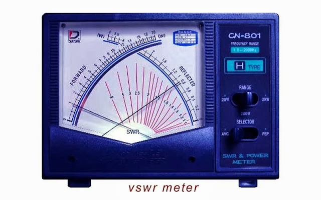
    There’s no better way to get your hands on gear—and stories—than at a hamfest. From Dayton’s legendary Hamvention to our own HAM-EX and York Region shows here in Ontario, these events are part swap meet, part social gathering, and part carnival. You might arrive looking for a particular SWR meter and leave with a trunk full of mystery boxes and a new circle of friends.

    2022 Hamilton Ontario Hamfest

    It’s that mix of technical curiosity and community that keeps this hobby alive. Long before online marketplaces and Discord chats, the hamfest was where you learned, traded, and laughed with people who spoke your language—literally and figuratively.

    The Supporting Cast

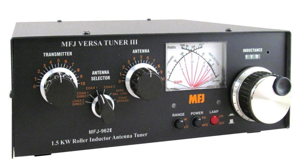
    A good station isn’t just a transceiver and a mic. Penny’s chapter reads like a love letter to the small but vital accessories that make a station run smoothly: the SWR meter, the dummy load, the antenna tuner, and those ingenious antenna switches that save you from untangling coax spaghetti. Each one has a role in keeping the station efficient, safe, and operational.

    His explanation of the antenna tuner—how it doesn’t “tune the antenna” at all but instead tricks your transmitter into seeing the load it wants—is a reminder of how much practical wisdom hides in this hobby.

    Antenna Tuner

    You learn theory, sure, but you also learn the gentle art of “coax diplomacy”: keeping your rig happy, your feedline loss low, and your neighbours blissfully unaware of their TV flickering every time you key up.

    A Final Thought

    In an age of plug-and-play everything, there’s something grounding—literally and figuratively—about building your own station. Each choice, from desk height to antenna orientation, reflects your habits and curiosity. You can buy the fanciest SDR on the market, but it won’t mean much until you’ve wrestled with grounding straps, tuned an antenna by ear, and smelled a resistor or two giving up the ghost.

    For me, that’s the heart of amateur radio: hands-on, imperfect, and wonderfully human. Every station tells a story—not just of frequencies and filters, but of persistence, learning, and connection.


    Bibliography

    [1] A. Penney, ‘Establishing and Equipping a Station’, presented at the RAC Basic Certificate Course, Radio Amateurs of Canada, Canada, Nov. 02, 2025. Accessed: Nov. 02, 2025. [Online]. Available: https://www.rac.ca/

  • Step-by-Step—Class 9

    Step-by-Step—Class 9

    This is post 12 of 28 in the series “Amateur Radio”

    Posts about my adventures in amateur radio.

    1. Step by step – 1st Class
    2. Step-by-Step – 2nd Class
    3. Amateur Radio Codes of Conduct
    4. Step-by-Step – 3rd Class
    5. Step-by-Step – Class 4a
    6. Step-by-Step – Classes 4b & 4c
    7. Step-by-Step—Class 5
    8. Step-by-Step—Class 6
    9. Step-by-Step—Class 7
    10. Step-by-Step—Class 8a
    11. Step-by-Step—Class 8b
    12. Step-by-Step—Class 9
    13. Step-by-Step—Class 10
    14. Step-by-step—Class 11
    15. A Modern Code of Conduct and Ethics for Amateur Radio
    16. Step-by-step—Class 12
    17. Step-by-step—Class 13
    18. Step-by-step—Class 14
    19. Step-by-step—Class 15
    20. Step-by-step—Class 16
    21. Step-by-step—Class 17
    22. Reflection: My Amateur Radio Journey So Far
    23. Authorized to Transmit
    24. Starting the Next Chapter: Advanced & CW
    25. Making Winlink, Pat, ARDOP and a Yaesu FTdx10 Work on an Apple Silicon Mac
    26. Winlink on Apple Silicon: The Files, Scripts and One-Click Launcher
    27. Whispers around the world
    28. Week 2 of CW Class

    From Vacuum Tubes to Transistors: A Personal Reflection on the Building Blocks of Modern Electronics

    Every once in a while, I come across a presentation that reminds me just how remarkable our journey in electronics has been. Al Penney’s “Diodes, Transistors and Tubes”, class 9 in the RAC Basic Qualification Course, is one of those — a concise, clear walk-through the history and physics that underpin virtually everything we take for granted in modern technology. [1]

    For anyone who’s ever built a circuit, troubleshot a control system, or simply wondered how a radio turns electromagnetic waves into sound, Al’s lecture is a reminder that the devices we use daily rest on a few elegant physical principles.

    Atoms, Electrons, and the Dance of Conductivity

    Al starts where all good electronics stories should: the atom. Protons, neutrons, and electrons — familiar from high school physics — become the players in a complex dance that determines whether a material is a conductor, an insulator, or something in between.

    Semiconductors sit in that fascinating “in-between” zone. By carefully introducing impurities, or doping, engineers can coax silicon or germanium into behaving predictably — letting electrons move when we want them to and stopping them when we don’t. That’s the foundation of everything from radio detectors to modern CPUs.

    The Simple Genius of the Diode

    The humble semiconductor diode, as Al explains, is just a P–N junction that lets current flow one way but not the other.

    Diagram of a PN junction diode showing both its physical structure and circuit symbol. The upper part depicts a semiconductor junction with p-type silicon on the left (anode) and n-type silicon on the right (cathode). The lower part shows the corresponding diode circuit symbol with the triangle representing current flow direction toward the vertical line, labelled with anode and cathode terminals.
    A p–n junction diode. The circuit symbol is also shown.
    By Raffamaiden – Own work, CC BY-SA 3.0, Link

    It’s the electronic equivalent of a check valve — elegantly simple, profoundly useful. With that one device, we can rectify AC into DC, demodulate radio signals, or stabilize voltage with a Zener diode.

    I’ve always appreciated how intuitively physical these analogies are. Whether you think of diodes as electrical check valves or semiconductors as engineered crystals, they connect the abstract world of physics with the very real world of current and voltage.

    Transistors: The Revolution in a Grain of Germanium

    A close-up photograph of the first transistor, the point-contact transistor invented at Bell Labs in 1947. The device is mounted on a clear acrylic stand, showing delicate wires connected to a small triangular germanium crystal on a metal base. Above the crystal, a bent wire spring applies pressure to the contacts. The setup includes fine leads and soldered connections, demonstrating the experimental nature of the original prototype used in early solid-state electronics research.
    The first transistor ever made, built by John Bardeen, William Shockley and Walter H. Brattain of Bell Labs in 1947. Original exhibited in Bell Laboratories. [2]
    Unitronic, CC BY-SA 3.0, via Wikimedia Commons
    Side-by-side image showing a point-contact transistor and its schematic diagram. On the left is a close-up photograph of an early germanium transistor with labeled components: emitter, collector, base, and a spring pressing a gold foil contact onto the germanium crystal mounted on a metal base. On the right is a simplified diagram showing the structure: a plastic wedge holding the emitter and collector contacts pressed onto a germanium substrate, with a thin razor cut between them to separate the two contacts, and labels for emitter, collector, base, spring, gold foil, and germanium.
    The first point-contact transistor is on the left. On the right is the schematic representation. 
    Image courtesy of AT&T.

    Then came the transistor — arguably the most transformative invention of the twentieth century. Al’s slides capture both the historical significance and the practical brilliance of that moment in 1947 when Bardeen and Brattain’s point-contact transistor first amplified a signal.

    Before that, we relied on vacuum tubes: glowing, fragile, power-hungry devices that filled radio chassis and computer rooms.

    A close-up photograph of an electronic vacuum tube, also known as a thermionic valve. The glass envelope is clear, showing the internal metal electrodes and grid structures. The tube has a metal base with several pins for insertion into a socket, and the top of the glass has a slightly darkened getter flash. The image is taken on a white background, highlighting the tube’s reflective surfaces and cylindrical shape.
    Vacuum Tube

    The transistor changed everything. It was small, efficient, rugged — and as Al notes, it enabled everything from portable radios to the computers that now run our world.

    Vintage 1940s Operadio Tube Amplifier [3]

    As someone who’s spent a career around control systems and functional safety, I find the transistor’s evolution from that sliver of germanium to today’s silicon MOSFETs a story of both science and engineering perseverance. Billions of transistors now sit on a chip smaller than your fingernail — each one still following the same basic principles first demonstrated in a Bell Labs lab bench.

    Amplifiers and the Art of Control

    One of Al’s most practical sections deals with amplification.

    Circuit diagram of a 25-watt audio amplifier using an integrated circuit (IC) TDA2040. The schematic shows input, power, and output stages. The audio input passes through capacitor C1 and resistor R1 to the non-inverting input of the IC (pin 1). Feedback is provided via resistors R2 and R3 and capacitor C2. Power supply decoupling capacitors C4 and C5 are connected to ±17V rails. The amplifier output drives a loudspeaker (LS1) through resistor R4 and capacitor C3.
    25 Watt Amplifier Circuit Diagram

    Whether we’re talking about boosting a microphone signal, driving a loudspeaker, or switching a safety relay, the amplifier’s purpose is the same — to make a small signal powerful enough to do useful work.

    Types of Transistors: Classification (BJT, JFET, MOSFET & IGBT) [4]

    Transistors and FETs handle this task differently, but the core idea is universal: use a small input to control a larger output. In machinery safety and control, this principle is evident everywhere — from sensor conditioning to PLC inputs and output stages, as well as pneumatics and hydraulics.

    Reflections on a Legacy of Innovation

    Al’s presentation closes with a nod to vacuum tubes — those glowing ancestors of the solid-state devices we know today. While they’ve been mostly replaced, they still hold a special place in audio and RF engineering for their distinctive performance characteristics.

    Vacuum tubes are still commonly used in specialized radio applications, particularly in high-power RF transmitters, including commercial radio and television broadcasting, amateur radio, and military communication systems. Their ability to handle high voltages, high power levels, and their linear amplification characteristics make them preferred in these settings where solid-state devices may be less reliable or unable to perform as well. Vacuum tubes are also valued for their durability in harsh environments, such as those with radiation or electromagnetic pulses (EMP), which is particularly important for military and aerospace applications.

    Key Radio Applications of Vacuum Tubes Today

    • High-Power Radio Transmitters: Commercial broadcast stations still use vacuum tubes for final power amplification due to their capacity to handle large RF power loads.
    • Amateur Radio Equipment: Many ham radio operators prefer tube-based transmitters for their superior signal handling, natural overload tolerance, and call sign authenticity in traditional equipment.
    • Military Communications: Vacuum tubes are preferred in certain military radios because of their robustness against EMP and radiation, ensuring reliable operation under extreme conditions.
    • Specialized Scientific and Industrial RF Systems: Vacuum tubes are used in some radar, industrial RF heating, and scientific instruments requiring high voltage and power.
    A British radio transmitter from the early 1920s, used for some of the first radio broadcasts by the British Broadcasting Corporation (BBC). The four early power triode valves (vacuum tubes) used in parallel resemble the 4 kW Marconi MT1 valves, developed by Marconi Co. engineer H. L. Round, which operated at 12,000 volts on the plate (anode). Blythe House Science Museum stores tour, London.
    By John Cummings – Own work, CC BY-SA 3.0, Link
    This beautiful example of home construction by Dick Stevens, W1QWJ, produces the “full gallon” (full, legally permitted power) on the 50 MHz band. The single tube is a 4CX1600B tetrode. [14]

    Additional Contemporary Uses Related to Radio

    • Vacuum tubes find niche roles in audio amplification equipment connected to radio receivers due to their characteristic sound.
    • Vacuum tube audiophile amplifiers are increasingly common, where their soft roll off when over-driven yield a much better sound than the harsh clipping that transistors give under similar conditions.
    • Some hybrid designs combine vacuum tube stages with solid-state components in modern radio equipment.
    Oilily A88 Vacuum Tube Integrated Amplifier, 45W+45W Class AB, EL34/KT88 Tube Amplifier with Triode & Ultra-Linear Mode, External Bias Adjustment, High-Fidelity Sound for Audiophiles (Black) [15]

    Thus, while transistors have largely replaced vacuum tubes in most consumer electronics, vacuum tubes remain essential in applications where their unique electrical and physical properties provide advantages that solid-state devices cannot fully match [5][6][7][8].

    Reading through this material reminded me that understanding where our technology comes from isn’t just nostalgic — it’s essential. Whether we’re designing safety systems, writing standards, or just tinkering in the shop, the principles that Al Penney lays out are as relevant today as they were when the first transistor clicked into life.

    In short: the story of diodes, transistors, and tubes isn’t just about components — it’s about curiosity, experimentation, and the human drive to control and harness electricity.

    Thanks, Al Penney (VO1NO), for reminding us how far we’ve come — and how much of that journey is still worth exploring.


    Bibliography

    [1] A. Penney, ‘Chapter 9 – Diodes, Transistors, and Tubes’, Radio Amateurs of Canada, Canada, Nov. 02, 2025. Accessed: Nov. 02, 2025. [Online]. Available: https://www.rac.ca/

    [2] J. T. Rubin, ‘The Invention of the Transistor’. Accessed: Oct. 29, 2025. [Online]. Available: https://www.juliantrubin.com/bigten/transistorexperiments.html

    [3] ‘Vintage 1940s Operadio Tube Amplifier Guitar Lap Steel Amp 5641 Speaker’, Worthpoint.com. Accessed: Nov. 01, 2025. [Online]. Available: https://www.worthpoint.com/worthopedia/vintage-1940s-operadio-tube-amplifier-4596304184

    [4] A. Singh, ‘Types of Transistors: Classification (BJT, JFET, MOSFET & IGBT)’, Hackatronic. Accessed: Nov. 01, 2025. [Online]. Available: https://www.hackatronic.com/types-of-transistors-classification-bjt-jfet-mosfet-igbt/

    [5] Vacuum Tubes: Complete Guide to Types, Applications & … https://www.blikai.com/blog/vacuumtube/vacuum-tubes-complete-guide-to-types-applications-modern-roles

    [6] Are Vacuum Tubes Still Used (& What Are They Used for)? https://pentalabs.com/blogs/tube-talk/are-vacuum-tubes-still-used

    [7] When Old is Gold: Harnessing the Power of Vintage … https://www.radiodesigngroup.com/blog/when-old-is-gold-harnessing-the-power-of-vintage-technology-for-modern-applications

    [8] Vacuum Tube Market Size & Share 2025-2032 https://www.360iresearch.com/library/intelligence/vacuum-tube

    [9] Brief Overview of Vacuum Tubes and Circuits https://www.bristolwatch.com/science/vacuum_tubes.htm

    [10] Vacuum tubes and modern uses for them : r/ECE https://www.reddit.com/r/ECE/comments/4hmi03/vacuum_tubes_and_modern_uses_for_them/

    [11] List of vacuum tubes https://en.wikipedia.org/wiki/List_of_vacuum_tubes

    [12] Modern Radio Technology Comparison to Tube Radio https://www.youtube.com/watch?v=GVXwsdsIyiI

    [13] Unlocking the Future of Vacuum Tube: Growth and Trends … https://www.marketreportanalytics.com/reports/vacuum-tube-376095

    [14] H. W. Silver, ‘Vacuum Tubes’, Nuts and Volts Magazine, no. November, pp. 8–11, 2017. Accessed: Nov. 01, 2025. [Online]. Available: https://www.nutsvolts.com/magazine/article/vacuum-tubes

    [15] ‘Oilily A88 Vacuum Tube Integrated Amplifier, 45W+45W Class AB, EL34/KT88 Tube Amplifier with Triode & Ultra-Linear Mode, External Bias Adjustment, High-Fidelity Sound for Audiophiles (Black)’, Tube Amplifier Reviews. Accessed: Nov. 01, 2025. [Online]. Available: https://tubeamplifierreviews.com/oilily-a88-vacuum-tube-integrated-amplifier-45w45w-class-ab-el34-kt88-tube-amplifier-with-triode-ultra-linear-mode-external-bias-adjustment-high-fidelity-sound-for-audiophiles-black/

  • Step-by-Step—Class 8b

    Step-by-Step—Class 8b

    This is post 11 of 28 in the series “Amateur Radio”

    Posts about my adventures in amateur radio.

    1. Step by step – 1st Class
    2. Step-by-Step – 2nd Class
    3. Amateur Radio Codes of Conduct
    4. Step-by-Step – 3rd Class
    5. Step-by-Step – Class 4a
    6. Step-by-Step – Classes 4b & 4c
    7. Step-by-Step—Class 5
    8. Step-by-Step—Class 6
    9. Step-by-Step—Class 7
    10. Step-by-Step—Class 8a
    11. Step-by-Step—Class 8b
    12. Step-by-Step—Class 9
    13. Step-by-Step—Class 10
    14. Step-by-step—Class 11
    15. A Modern Code of Conduct and Ethics for Amateur Radio
    16. Step-by-step—Class 12
    17. Step-by-step—Class 13
    18. Step-by-step—Class 14
    19. Step-by-step—Class 15
    20. Step-by-step—Class 16
    21. Step-by-step—Class 17
    22. Reflection: My Amateur Radio Journey So Far
    23. Authorized to Transmit
    24. Starting the Next Chapter: Advanced & CW
    25. Making Winlink, Pat, ARDOP and a Yaesu FTdx10 Work on an Apple Silicon Mac
    26. Winlink on Apple Silicon: The Files, Scripts and One-Click Launcher
    27. Whispers around the world
    28. Week 2 of CW Class

    Back to Basics: Practical Antennas and the Beauty of Simplicity

    When I first started in electronics back in the mid-’80s, one of the first things I learned was that good design doesn’t always mean complex design. Nowhere is that truer than with antennas. Chapter 8B of the RAC Basic Certificate Course reminded me of something many of us tend to forget: the simplest antennas often work the best.

    (more…)
  • Step-by-Step—Class 6

    Step-by-Step—Class 6

    This is post 8 of 28 in the series “Amateur Radio”

    Posts about my adventures in amateur radio.

    1. Step by step – 1st Class
    2. Step-by-Step – 2nd Class
    3. Amateur Radio Codes of Conduct
    4. Step-by-Step – 3rd Class
    5. Step-by-Step – Class 4a
    6. Step-by-Step – Classes 4b & 4c
    7. Step-by-Step—Class 5
    8. Step-by-Step—Class 6
    9. Step-by-Step—Class 7
    10. Step-by-Step—Class 8a
    11. Step-by-Step—Class 8b
    12. Step-by-Step—Class 9
    13. Step-by-Step—Class 10
    14. Step-by-step—Class 11
    15. A Modern Code of Conduct and Ethics for Amateur Radio
    16. Step-by-step—Class 12
    17. Step-by-step—Class 13
    18. Step-by-step—Class 14
    19. Step-by-step—Class 15
    20. Step-by-step—Class 16
    21. Step-by-step—Class 17
    22. Reflection: My Amateur Radio Journey So Far
    23. Authorized to Transmit
    24. Starting the Next Chapter: Advanced & CW
    25. Making Winlink, Pat, ARDOP and a Yaesu FTdx10 Work on an Apple Silicon Mac
    26. Winlink on Apple Silicon: The Files, Scripts and One-Click Launcher
    27. Whispers around the world
    28. Week 2 of CW Class

    Riding the Waves: Reflections on Radio Propagation

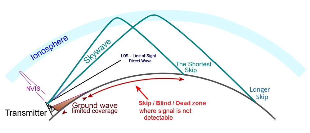
    This week’s class on radio-wave propagation took me right back to my roots. It’s hard not to smile when I see diagrams of skywaves, ground waves, and skip zones — things I first learned about nearly forty years ago at Sheridan College, when we were still using analog oscilloscopes and scientific calculators. Back then, I was an electronics engineering technology student just getting ready to start my career, and the idea that invisible waves could circle the globe felt almost magical.

    Now, as I sit in class once again — decades later, after a long career in electronics and electrical control system design — I see those same principles through a different lens. What once seemed like mysterious phenomena now feel like old friends whose habits I know well. The theory hasn’t changed, even though the tools and applications have evolved beyond what I could have imagined in 1985.

    From Spark-Gap to Skywave

    The story of radio propagation is as much about curiosity as it is about science. When Guglielmo Marconi proved in 1901 that a wireless signal could cross the Atlantic, he didn’t know why it worked — only that it did. He thought the waves were following the Earth’s curve, but in reality, they were bouncing off the ionosphere — a discovery that wouldn’t be fully understood for decades.

    That experiment, conducted from Signal Hill in St. John’s, Newfoundland, still captures my imagination. It’s a reminder of how experimentation often leads the theory, and how the physics that govern our communication systems today are the same ones that guided those first transatlantic dots and dashes of Morse code.

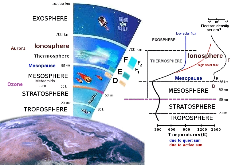
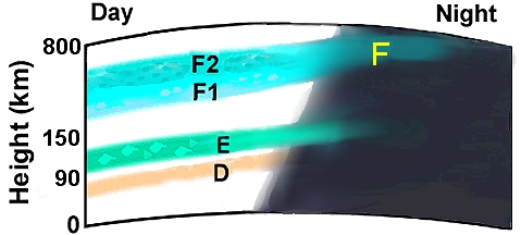
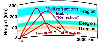
    The Ionosphere: A Living Mirror

    Of all the layers of the atmosphere, the ionosphere remains the most fascinating. The D, E, and F layers — invisible, dynamic, and ever-changing — are what make global communication possible.

    A schematic cross-section of Earth’s atmosphere and ionosphere: The left side shows the Earth at the bottom with concentric transparent bands representing atmospheric layers (troposphere near the surface, then stratosphere, mesosphere, thermosphere, and exosphere at the top). On the right side, a simplified graph overlays region boundaries labelled D, E, and F, with dashed lines indicating locations within the thermosphere and upper mesosphere. Temperature and/or density axes are implied, indicating an increase in altitude upward to approximately 10,000 km. The graphic emphasizes that the ionosphere (regions D → E → F) lies within the thermosphere/upper atmosphere.
    The Ionosphere (Thermosphere) is part of Earth’s Atmosphere. The Thermosphere is characterized by very high temperatures ranging from 550 to over 1300 degrees Kelvin due to the solar EUV. [1]
    image: qsl.net
    A stylized diagram showing the ionospheric regions over the Earth’s surface during day and night: On the left side (“day”), three colored horizontal bands labelled D (~60-90 km), E (~90-150 km), and F (~150-≈600 km) ascend upward from the Earth’s surface. On the right side (“night”), only the F region remains prominent (labelled “F”), while the D and E bands are faint or absent. Arrows indicate solar-ionization (incoming from the sun-lit side) and recombination (on the night side). The figure emphasizes how free-electron density varies by region and time of day.
    Ionospheric regions illustration [1]
    image: qsl.net

    During the day, the D layer absorbs low-frequency signals, muting AM stations that roar back to life at sunset. The higher F layers, split into F1 and F2 in daylight, refract HF signals over thousands of kilometres, bending them back toward Earth like a mirror made of charged particles. [1], [3]

    A schematic diagram showing three distinct radio-wave propagation paths between a transmitter and a distant receiver:
• On the left, a straight line labelled “Line-of-Sight (LOS)” travels directly from the transmitting antenna to the receiving antenna above the Earth’s surface, implying a direct path without bending.
• In the middle, a path labelled “Ground Wave / Surface Wave” follows along the contour of the Earth’s surface (curving slightly), indicating a wave that hugs the ground and travels beyond the visual horizon.
• On the right, a curved upward-then-downward path labelled “Sky-Wave / Ionospheric Refraction” leaves the transmitter at a low angle, arcs upward to the ionosphere, bends (or is refracted) back toward the Earth, and lands at the receiver far beyond the horizon. In the space between the ground-wave and sky-wave paths is the “skip zone” (a region of no reception) indicated by shading or dashed lines. The diagram is set against a stylized cross-section of the Earth and atmosphere, with altitude increasing upward and horizontal distance along the bottom.
    Ionospheric reflections
    image: qsl.net [3]

    Even after years of working with EMI and high-frequency noise in control systems, it still amazes me how the same physics in a factory floor’s PLC cabinet also govern how a signal from halfway around the world reaches a simple dipole antenna in my backyard.

    Of Sunspots, Solar Flux, and the Unseen Weather Above

    As engineers, we tend to think of “weather” as something that affects reliability through temperature or humidity. But this week’s class reminded me that space weather plays an equally critical role. Solar flares, coronal mass ejections, and sunspots — the restless activity of our nearest star — shape the ionosphere daily [2], [5].

    The Dominion Radio Astrophysical Observatory in Penticton, BC, has been measuring the Sun’s radio emissions at 2800 MHz since the 1940s, producing the Solar Flux Index we still rely on. Seeing that connection between a Canadian observatory, solar physics, and real-world radio performance renewed my appreciation for how deeply our communications depend on phenomena far beyond our control.

    Skip Zones, Fading, and the Fragile Nature of Connection

    In my work over the years, I’ve seen signal dropouts caused by everything from ground loops to induction noise, but ionospheric fading has a kind of poetry to it. The way signals strengthen and vanish as the ionosphere shifts with time and sunlight reminds me that all communication — whether through copper, fibre, or free space — is ultimately about timing and conditions.

    Overview of HF Propagation Modes
    image: qsl.net [3]

    Skip zones, backscatter, and multipath effects are more than textbook curiosities; they’re metaphors for the real-world challenge of designing systems that perform reliably despite an unpredictable environment. Our ability to predict, compensate for, and even exploit those effects is a testament to a century of accumulated engineering wisdom.

    NVIS and the Modern Relevance of Propagation

    Near Vertical Incidence Skywave (NVIS) propagation especially caught my attention. It’s used today for short-range HF communication, where terrain or disasters might block line-of-sight signals. I couldn’t help but think how that same principle could apply to robust emergency communications or even industrial networks in remote regions.

    Approximate NVIS Signal Range [4]
    image: hamradiooutsidethebox.ca

    NVIS signals are propagated at a high elevation (greater than 60°). They are reflected down from the ionosphere (principally the F2 layer) over an area of a few hundred kilometres from the source. [4]

    Using trigonometric calculations, we can estimate the NVIS coverage to be about 350 kilometres. Because the diagram represents a two-dimensional view, it’s essential to understand that this range extends equally in all directions from the transmitting station. In other words, if we imagine a circle centred on the transmitter with a radius of 350 kilometres, any receiver positioned within that circle should be able to detect the NVIS signal.

    Despite all our modern connectivity, there’s still a place for understanding how nature itself moves information from one point to another.

    Closing Thoughts

    For me, studying propagation again isn’t about relearning the formulas — it’s about rediscovering the elegance behind them. The same electromagnetic principles that may have carried Marconi’s letter “S” across the Atlantic in 1901 still underpin the wireless links in a factory, the telemetry in a wind farm, or the Wi-Fi in our homes.

    After four decades in the field, it’s humbling to be reminded that no matter how advanced our technology becomes, we’re still riding the same waves — reflections from the same sky, governed by the same physics, and inspired by the same human drive to connect across distance.


    References

    [1] D. Tal, “Region vs. Layer: Earth’s Atmosphere and Ionosphere”. Accessed: Oct. 10, 2025. [Online]. Available: https://www.qsl.net/4x4xm/Region-vs-Layer-Earth’s-Atmosphere-and-Ionosphere.htm

    [2] ‘Space Weather’, spaceweather.com. Accessed: Oct. 10, 2025. [Online]. Available: https://www.spaceweather.com

    [3] D. Tal, ‘Skywave Propagation Basics’, Understanding HF Skywave Propagation. Accessed: Oct. 21, 2025. [Online]. Available: https://www.qsl.net/4x4xm/HF-Propagation.htm

    [4] John VA3KOT, ‘The NVIS Illusion’, Ham Radio Outside the Box. Accessed: Oct. 21, 2025. [Online]. Available: https://hamradiooutsidethebox.ca/2023/06/19/the-nvis-illusion/

    [5] N. R. C. Government of Canada, ‘Current regional magnetic conditions’. Accessed: Oct. 21, 2025. [Online]. Available: https://www.spaceweather.gc.ca/forecast-prevision/short-court/regional/sr-1-en.php?region=ott&mapname=east_n_america

  • Step-by-Step—Class 5

    Step-by-Step—Class 5

    This is post 7 of 28 in the series “Amateur Radio”

    Posts about my adventures in amateur radio.

    1. Step by step – 1st Class
    2. Step-by-Step – 2nd Class
    3. Amateur Radio Codes of Conduct
    4. Step-by-Step – 3rd Class
    5. Step-by-Step – Class 4a
    6. Step-by-Step – Classes 4b & 4c
    7. Step-by-Step—Class 5
    8. Step-by-Step—Class 6
    9. Step-by-Step—Class 7
    10. Step-by-Step—Class 8a
    11. Step-by-Step—Class 8b
    12. Step-by-Step—Class 9
    13. Step-by-Step—Class 10
    14. Step-by-step—Class 11
    15. A Modern Code of Conduct and Ethics for Amateur Radio
    16. Step-by-step—Class 12
    17. Step-by-step—Class 13
    18. Step-by-step—Class 14
    19. Step-by-step—Class 15
    20. Step-by-step—Class 16
    21. Step-by-step—Class 17
    22. Reflection: My Amateur Radio Journey So Far
    23. Authorized to Transmit
    24. Starting the Next Chapter: Advanced & CW
    25. Making Winlink, Pat, ARDOP and a Yaesu FTdx10 Work on an Apple Silicon Mac
    26. Winlink on Apple Silicon: The Files, Scripts and One-Click Launcher
    27. Whispers around the world
    28. Week 2 of CW Class

    From Sparks to Software: Reflections on Waves, Wavelengths, and the Spirit of Radio

    Every so often, a class reminds me that the fundamentals never really change. This week’s topic — Waves, Wavelength, Frequency, and Bands — was a trip back in time for me. As someone who trained as an electronics engineering technologist in the 1980s, this material feels like old territory. Yet, revisiting it in today’s context, with modern software-defined radios (SDRs) and digital signal processing, highlights just how enduring these basic principles are.

    The Timeless Language of Waves

    The lecture opened with the essentials: amplitude, wavelength, and frequency — the vocabulary of every waveform, whether it’s a sound wave in air or a radio wave racing through space. Back then, we learned these on oscilloscopes with green phosphor traces, adjusting time bases and triggering circuits to freeze those elegant sine waves in time. Today, the same principles remain, but the scopes are digital, and the waves are simulated, captured, and analyzed by software.

    A diagram of the electromagnetic spectrum, showing various properties across the range of frequencies and wavelengths.
    Image: Inductiveload, Wikimedia Commons

    What hasn’t changed is the relationship between wavelength and frequency — the beautiful simplicity of ( c = f \λ ), where the speed of light ties them together. It’s still the same 300 × 106 metres per second in free space, as it was for Heinrich Hertz when he first proved Maxwell’s equations right. The numbers might scale from kilohertz to gigahertz now, but the physics hasn’t changed a bit.

    Band NameAbbr.ITU bandFrequencyWavelength
    Extremely low frequencyELF13–30 Hz100,000–10,000 km
    Super low frequencySLF230–300 Hz10,000–1,000 km
    Ultra low frequencyULF3300–3,000 Hz1,000–100 km
    Very low frequencyVLF43–30 kHz100–10 km
    Low frequencyLF530–300 kHz10–1 km
    Medium frequencyMF6300–3,000 kHz1,000–100 m
    High frequencyHF73–30 MHz100–10 m
    Very high frequencyVHF830–300 MHz10–1 m
    Ultra high frequencyUHF9300–3,000 MHz100–10 cm
    Super high frequencySHF103–30 GHz10–1 cm
    Extremely high frequencyEHF1130–300 GHz10–1 mm
    Terahertz or tremendously high frequencyTHF12300–3,000 GHz1–0.1 mm
    Band names
    [13]

    A Short History of Long Waves

    Thinking about waves and bands always takes me back to the early history of radio — to the days of spark-gap transmitters, longwave Morse signals, and men like Hertz, Marconi, and Fessenden. Those pioneers were dealing with kilohertz frequencies, with antennas and capacitors the size of ships, yet they were manipulating the same invisible medium we use today.

    Marconi’s Antenna Towers, Glace Bay, Nova Scotia. The four 200-foot wooden latticework towers shown supported an inverted pyramid of antenna wires not visible in the photo.
    Marconi Antenna Array Structure, 1907

    I’m pretty sure my neighbours would be unhappy with me if I built an antenna array that resembled Marconi’s Glace Bay installation!

    The circuit diagram of the December 1901 Poldhu transmitter in J.A. Fleming’s handwriting.

    By 1907, the Marconi station at Glace Bay, Nova Scotia, was operating on remarkably low frequencies for its time — around 70 kHz. That range was chosen for the transatlantic service linking Glace Bay with Clifden, Ireland, inaugurated in October 1907.

    Earlier experiments at the site had been conducted on higher frequencies — roughly 182 kHz in 1902 and 272 kHz for some later trials — but Marconi’s engineers soon discovered that lower frequencies provided far greater reliability over long distances. By 1907, they had moved down to around 70 kHz, and eventually as low as 45 kHz.

    These very long wavelengths (VLF) proved ideal for transatlantic work. The signals could travel enormous distances, reflecting between the Earth and the ionosphere, and remained stable both day and night — something that higher frequencies of the day couldn’t achieve. Considering the limits of early transmitters and receivers, this was an extraordinary technical accomplishment and a milestone in the development of reliable global communication.

    First Transatlantic Radio Service, October 17, 1907

    In the photo above, Marconi Operator L.R. Johnstone is shown transmitting the first official messages of the commercial wireless telegraph service from Marconi Towers, near Glace Bay, Nova Scotia, to Clifden, Ireland, on October 17, 1907. Ten thousand words were exchanged between the stations on the first day of operation.

    Marconi rotary spark discharger
    image: Cape Breton Wireless Heritage Society

    The rotary spark discharger was the heart of the spark transmitter at Marconi Towers. In the upper-right background, the three large ring-shaped loops are the three turns of the antenna transformer’s primary coil, which fed the spark’s electrical energy into the high-mounted antenna.

    Historical Photo of Marconi Wireless Site and Towers in Glace Bay, Nova Scotia, Canada.
    See page for author, Public domain, via Wikimedia Commons.
    Coal-fired boilers in the power house at Marconi Towers produced steam for the main steam engine and alternator.
    image: Cape Breton Wireless Heritage Society

    At the Marconi station in Glace Bay, Nova Scotia, six steam boilers powered dynamos that generated the 15 kV power supply, which charged a capacitor composed of 288 metal sheets, each measuring 60 feet by 20 feet, separated by approximately 6 inches. The sheets were suspended from rafters at the top of the building and hung vertically almost to ground level. This capacitor (or “condenser,” as it was initially called) occupied most of the 160-foot-long transmitter building. As a result, the building became known as the condenser building.

    Main operating building of Marconi Wireless Station, ca. 1912.
    Collection of Port Morien Station, ca. 1912 / Collection de la station de Port Morien, vers 1912.

    This extensive array of plates offered only 1.7 microfarads of capacitance, with a voltage rating of 15 kilovolts. An “air-insulated” design was selected over a more compact glass dielectric design because it was relatively trouble-free and easy to build using locally available materials. If a draft caused the plates to shift and short-circuit, the “spot-welded” plates could be knocked apart with a sledgehammer.

    Marconi’s Condenser (Capacitor) at Glace Bay, Nova Scotia

    One story that sticks in my mind is Weather Station Kurt, a German automatic transmitter secretly placed in Labrador during the Second World War. It operated on 3940 kHz — smack in what we now think of as the amateur 80 m band — sending weather reports back to Germany every few hours. Even in wartime, radio’s reach was both strategic and scientific, and its physics — the propagation of electromagnetic waves through atmosphere and ionosphere — governed everything.

    From Resonant Circuits to Software Radios

    Interaction between Capacitive and Inductive reactance and the resonance point — Slide by Al Penny VO1NO

    When I first learned about LC circuits, we tuned them with physical coils and capacitors, feeling resonance through the sound in a speaker or the flicker on a meter. The “bands” we talked about then — HF, VHF, UHF — were as much about practical limitations as they were about regulation. Antenna length, wavelength, and atmospheric reflection all dictated what was possible.

    Today, when I look at a modern software-defined radio (SDR), I find it astonishing to think that an entire superheterodyne receiver now fits in a USB drive. Instead of a coil and a capacitor, we use algorithms to shift and filter signals in code. But the foundation — waves, frequencies, and harmonics — is the same. Whether it’s a spark-gap transmitter, a vacuum-tube superhet, or a LimeSDR, every one of them lives by the same electromagnetic laws.

    Why It Still Matters

    There’s a certain poetry in knowing that a 7 MHz signal — the classic 40 m amateur band — still bounces off the ionosphere just as it did when I first listened to shortwave broadcasts as a teenager. The gear has changed; the spectrum hasn’t. Even in a world dominated by Wi-Fi, Bluetooth, and cellular links operating in gigahertz ranges, it all still comes down to waves oscillating in time and space.

    So while the students around me might be seeing this material for the first time, I find myself smiling at how familiar it feels. The math is old, the physics immutable, and yet the applications keep evolving. From sparks to software, from the hiss of AM static to the crisp digital decoding of an SDR waterfall, it’s all the same story — one wave at a time.

    Looking Ahead

    As the course continues, I’m looking forward to diving deeper into how these timeless wave fundamentals shape the communication technologies we rely on every day. Understanding them through both the lens of experience and modern tools like SDRs bridges the gap between the analog world in which I first learned and the digital systems that define today’s engineering practice. It’s a reminder that while technology evolves, the language of physics remains beautifully consistent — and that makes every new concept feel like an old friend revisited.


    References

    [1] Marconi – Krause House Info-Research Solutions

    [2] On this day in 1907

    [3] List of Marconi wireless stations

    [4] Guglielmo Marconi

    [5] List of Marconi wireless stations – Wikiwand

    [6] Frequency Spectrum Management Overview

    [7] Radio’s First Message – Fessenden and Marconi

    [8] An Historical and Technological Survey

    [9] ULTRA TCS – Canadian Marconi History

    [10] VE1DEW – Callsign Lookup by QRZ Ham Radio

    [11] M. Rosano, “Throwback Thursday: Nazi weather station in Labrador”, Canadian Geographic. 2015. Available: https://canadiangeographic.ca/articles/throwback-thursday-nazi-weather-station-in-labrador/ [Accessed: 2025-10-16]

    [12] ‘The First Transatlantic Wireless Stations in Cape Breton’, Cape Breton Wireless Heritage Society. Accessed: Oct. 13, 2025. [Online]. Available: http://www.cbwireless.ednet.ns.ca/cbwirelessp3.html

    [13] Rajiv, ‘Radio Frequency Bands’, RF Page. Accessed: Dec. 07, 2025. [Online]. Available: https://www.rfpage.com/what-are-radio-frequency-bands-and-its-uses/