Last updated on 2025-11-07 at 11:34 EST (UTC-05:00)
Riding the Waves: Reflections on Radio Propagation
This week’s class on radio-wave propagation took me right back to my roots. It’s hard not to smile when I see diagrams of skywaves, ground waves, and skip zones — things I first learned about nearly forty years ago at Sheridan College, when we were still using analog oscilloscopes and scientific calculators. Back then, I was an electronics engineering technology student just getting ready to start my career, and the idea that invisible waves could circle the globe felt almost magical.
Now, as I sit in class once again — decades later, after a long career in electronics and electrical control system design — I see those same principles through a different lens. What once seemed like mysterious phenomena now feel like old friends whose habits I know well. The theory hasn’t changed, even though the tools and applications have evolved beyond what I could have imagined in 1985.
From Spark-Gap to Skywave
The story of radio propagation is as much about curiosity as it is about science. When Guglielmo Marconi proved in 1901 that a wireless signal could cross the Atlantic, he didn’t know why it worked — only that it did. He thought the waves were following the Earth’s curve, but in reality, they were bouncing off the ionosphere — a discovery that wouldn’t be fully understood for decades.
That experiment, conducted from Signal Hill in St. John’s, Newfoundland, still captures my imagination. It’s a reminder of how experimentation often leads the theory, and how the physics that govern our communication systems today are the same ones that guided those first transatlantic dots and dashes of Morse code.
The Ionosphere: A Living Mirror
Of all the layers of the atmosphere, the ionosphere remains the most fascinating. The D, E, and F layers — invisible, dynamic, and ever-changing — are what make global communication possible.
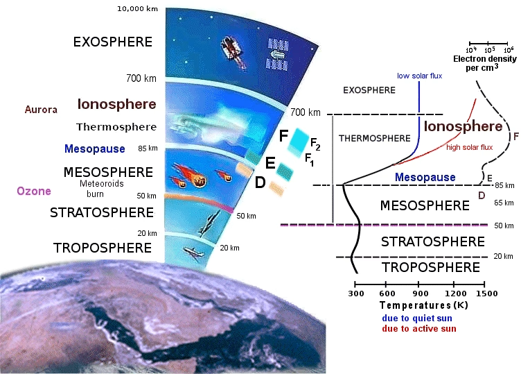
image: qsl.net
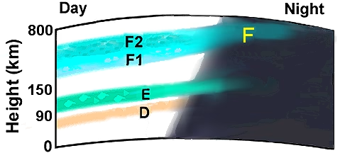
image: qsl.net
During the day, the D layer absorbs low-frequency signals, muting AM stations that roar back to life at sunset. The higher F layers, split into F1 and F2 in daylight, refract HF signals over thousands of kilometres, bending them back toward Earth like a mirror made of charged particles. [1], [3]
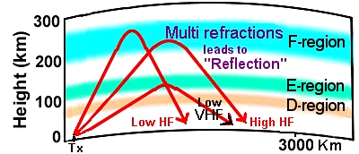
image: qsl.net [3]
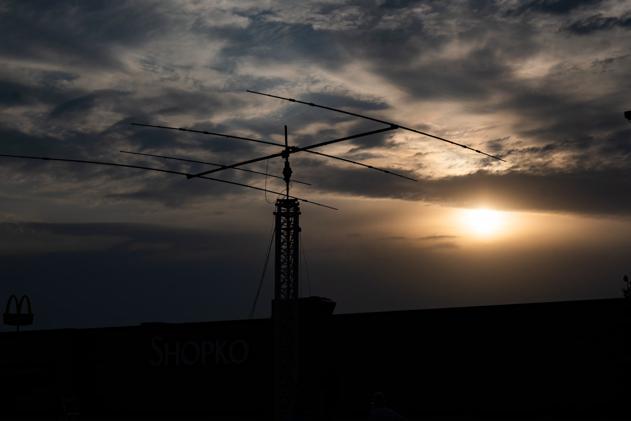
Even after years of working with EMI and high-frequency noise in control systems, it still amazes me how the same physics in a factory floor’s PLC cabinet also govern how a signal from halfway around the world reaches a simple dipole antenna in my backyard.
Of Sunspots, Solar Flux, and the Unseen Weather Above
As engineers, we tend to think of “weather” as something that affects reliability through temperature or humidity. But this week’s class reminded me that space weather plays an equally critical role. Solar flares, coronal mass ejections, and sunspots — the restless activity of our nearest star — shape the ionosphere daily [2], [5].
The Dominion Radio Astrophysical Observatory in Penticton, BC, has been measuring the Sun’s radio emissions at 2800 MHz since the 1940s, producing the Solar Flux Index we still rely on. Seeing that connection between a Canadian observatory, solar physics, and real-world radio performance renewed my appreciation for how deeply our communications depend on phenomena far beyond our control.
Skip Zones, Fading, and the Fragile Nature of Connection
In my work over the years, I’ve seen signal dropouts caused by everything from ground loops to induction noise, but ionospheric fading has a kind of poetry to it. The way signals strengthen and vanish as the ionosphere shifts with time and sunlight reminds me that all communication — whether through copper, fibre, or free space — is ultimately about timing and conditions.
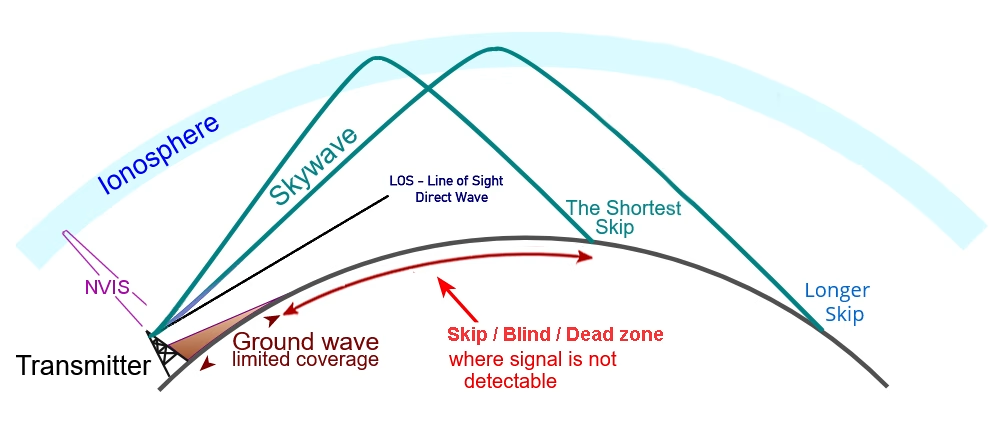
image: qsl.net [3]
Skip zones, backscatter, and multipath effects are more than textbook curiosities; they’re metaphors for the real-world challenge of designing systems that perform reliably despite an unpredictable environment. Our ability to predict, compensate for, and even exploit those effects is a testament to a century of accumulated engineering wisdom.
NVIS and the Modern Relevance of Propagation
Near Vertical Incidence Skywave (NVIS) propagation especially caught my attention. It’s used today for short-range HF communication, where terrain or disasters might block line-of-sight signals. I couldn’t help but think how that same principle could apply to robust emergency communications or even industrial networks in remote regions.
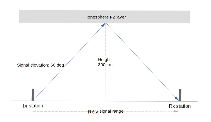
image: hamradiooutsidethebox.ca
NVIS signals are propagated at a high elevation (greater than 60°). They are reflected down from the ionosphere (principally the F2 layer) over an area of a few hundred kilometres from the source. [4]
Using trigonometric calculations, we can estimate the NVIS coverage to be about 350 kilometres. Because the diagram represents a two-dimensional view, it’s essential to understand that this range extends equally in all directions from the transmitting station. In other words, if we imagine a circle centred on the transmitter with a radius of 350 kilometres, any receiver positioned within that circle should be able to detect the NVIS signal.
Despite all our modern connectivity, there’s still a place for understanding how nature itself moves information from one point to another.
Closing Thoughts
For me, studying propagation again isn’t about relearning the formulas — it’s about rediscovering the elegance behind them. The same electromagnetic principles that may have carried Marconi’s letter “S” across the Atlantic in 1901 still underpin the wireless links in a factory, the telemetry in a wind farm, or the Wi-Fi in our homes.
After four decades in the field, it’s humbling to be reminded that no matter how advanced our technology becomes, we’re still riding the same waves — reflections from the same sky, governed by the same physics, and inspired by the same human drive to connect across distance.
References
[1] D. Tal, “Region vs. Layer: Earth’s Atmosphere and Ionosphere”. Accessed: Oct. 10, 2025. [Online]. Available: https://www.qsl.net/4x4xm/Region-vs-Layer-Earth’s-Atmosphere-and-Ionosphere.htm
[2] ‘Space Weather’, spaceweather.com. Accessed: Oct. 10, 2025. [Online]. Available: https://www.spaceweather.com
[3] D. Tal, ‘Skywave Propagation Basics’, Understanding HF Skywave Propagation. Accessed: Oct. 21, 2025. [Online]. Available: https://www.qsl.net/4x4xm/HF-Propagation.htm
[4] John VA3KOT, ‘The NVIS Illusion’, Ham Radio Outside the Box. Accessed: Oct. 21, 2025. [Online]. Available: https://hamradiooutsidethebox.ca/2023/06/19/the-nvis-illusion/
[5] N. R. C. Government of Canada, ‘Current regional magnetic conditions’. Accessed: Oct. 21, 2025. [Online]. Available: https://www.spaceweather.gc.ca/forecast-prevision/short-court/regional/sr-1-en.php?region=ott&mapname=east_n_america
Leave a Reply