From Vacuum Tubes to Transistors: A Personal Reflection on the Building Blocks of Modern Electronics

Every once in a while, I come across a presentation that reminds me just how remarkable our journey in electronics has been. Al Penney’s “Diodes, Transistors and Tubes”, class 9 in the RAC Basic Qualification Course, is one of those — a concise, clear walk-through the history and physics that underpin virtually everything we take for granted in modern technology. [1]

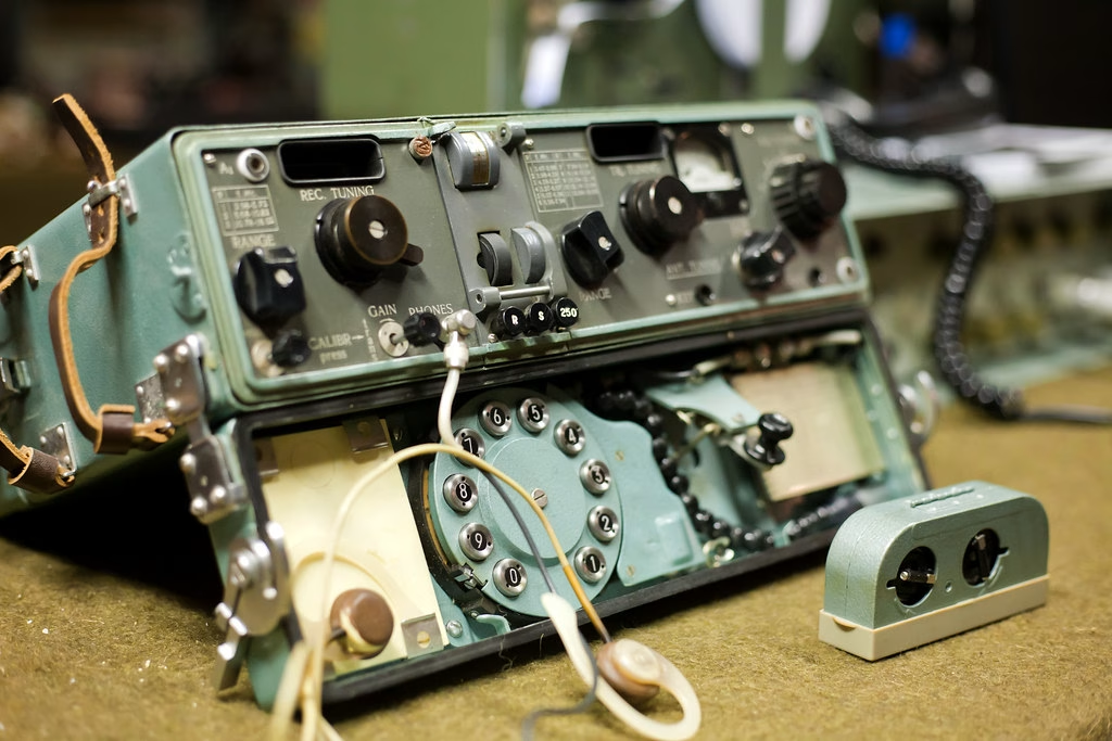
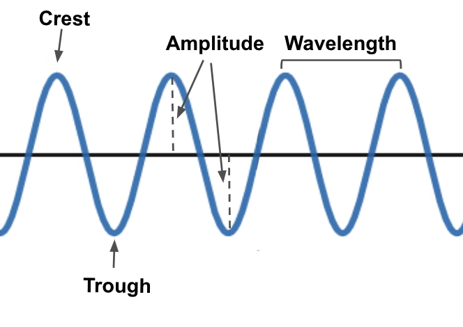
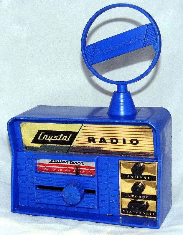
For anyone who’s ever built a circuit, troubleshot a control system, or simply wondered how a radio turns electromagnetic waves into sound, Al’s lecture is a reminder that the devices we use daily rest on a few elegant physical principles.

Atoms, Electrons, and the Dance of Conductivity

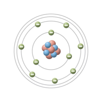
Al starts where all good electronics stories should: the atom. Protons, neutrons, and electrons — familiar from high school physics — become the players in a complex dance that determines whether a material is a conductor, an insulator, or something in between.

Semiconductors sit in that fascinating “in-between” zone. By carefully introducing impurities, or doping, engineers can coax silicon or germanium into behaving predictably — letting electrons move when we want them to and stopping them when we don’t. That’s the foundation of everything from radio detectors to modern CPUs.

The Simple Genius of the Diode

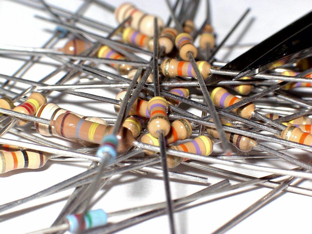
The humble semiconductor diode, as Al explains, is just a P–N junction that lets current flow one way but not the other.

It’s the electronic equivalent of a check valve — elegantly simple, profoundly useful. With that one device, we can rectify AC into DC, demodulate radio signals, or stabilize voltage with a Zener diode.

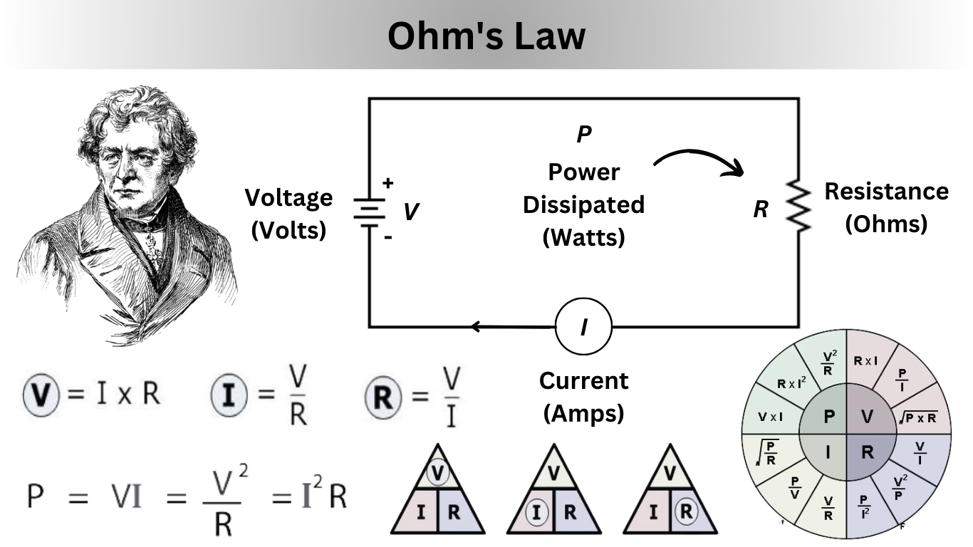
I’ve always appreciated how intuitively physical these analogies are. Whether you think of diodes as electrical check valves or semiconductors as engineered crystals, they connect the abstract world of physics with the very real world of current and voltage.

Transistors: The Revolution in a Grain of Germanium

Then came the transistor — arguably the most transformative invention of the twentieth century. Al’s slides capture both the historical significance and the practical brilliance of that moment in 1947 when Bardeen and Brattain’s point-contact transistor first amplified a signal.

Before that, we relied on vacuum tubes: glowing, fragile, power-hungry devices that filled radio chassis and computer rooms.

The transistor changed everything. It was small, efficient, rugged — and as Al notes, it enabled everything from portable radios to the computers that now run our world.

As someone who’s spent a career around control systems and functional safety, I find the transistor’s evolution from that sliver of germanium to today’s silicon MOSFETs a story of both science and engineering perseverance. Billions of transistors now sit on a chip smaller than your fingernail — each one still following the same basic principles first demonstrated in a Bell Labs lab bench.

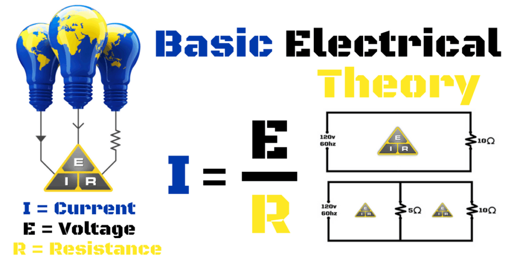
Amplifiers and the Art of Control

One of Al’s most practical sections deals with amplification.

Whether we’re talking about boosting a microphone signal, driving a loudspeaker, or switching a safety relay, the amplifier’s purpose is the same — to make a small signal powerful enough to do useful work.

Transistors and FETs handle this task differently, but the core idea is universal: use a small input to control a larger output. In machinery safety and control, this principle is evident everywhere — from sensor conditioning to PLC inputs and output stages, as well as pneumatics and hydraulics.

Reflections on a Legacy of Innovation

Al’s presentation closes with a nod to vacuum tubes — those glowing ancestors of the solid-state devices we know today. While they’ve been mostly replaced, they still hold a special place in audio and RF engineering for their distinctive performance characteristics.

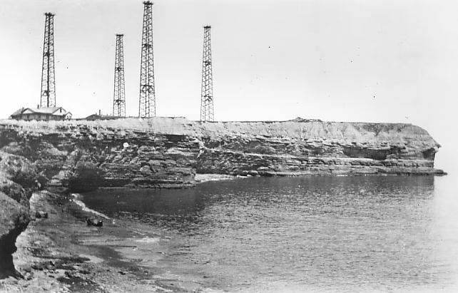
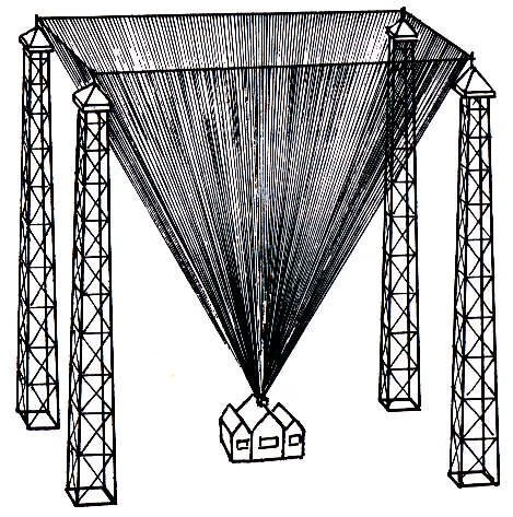
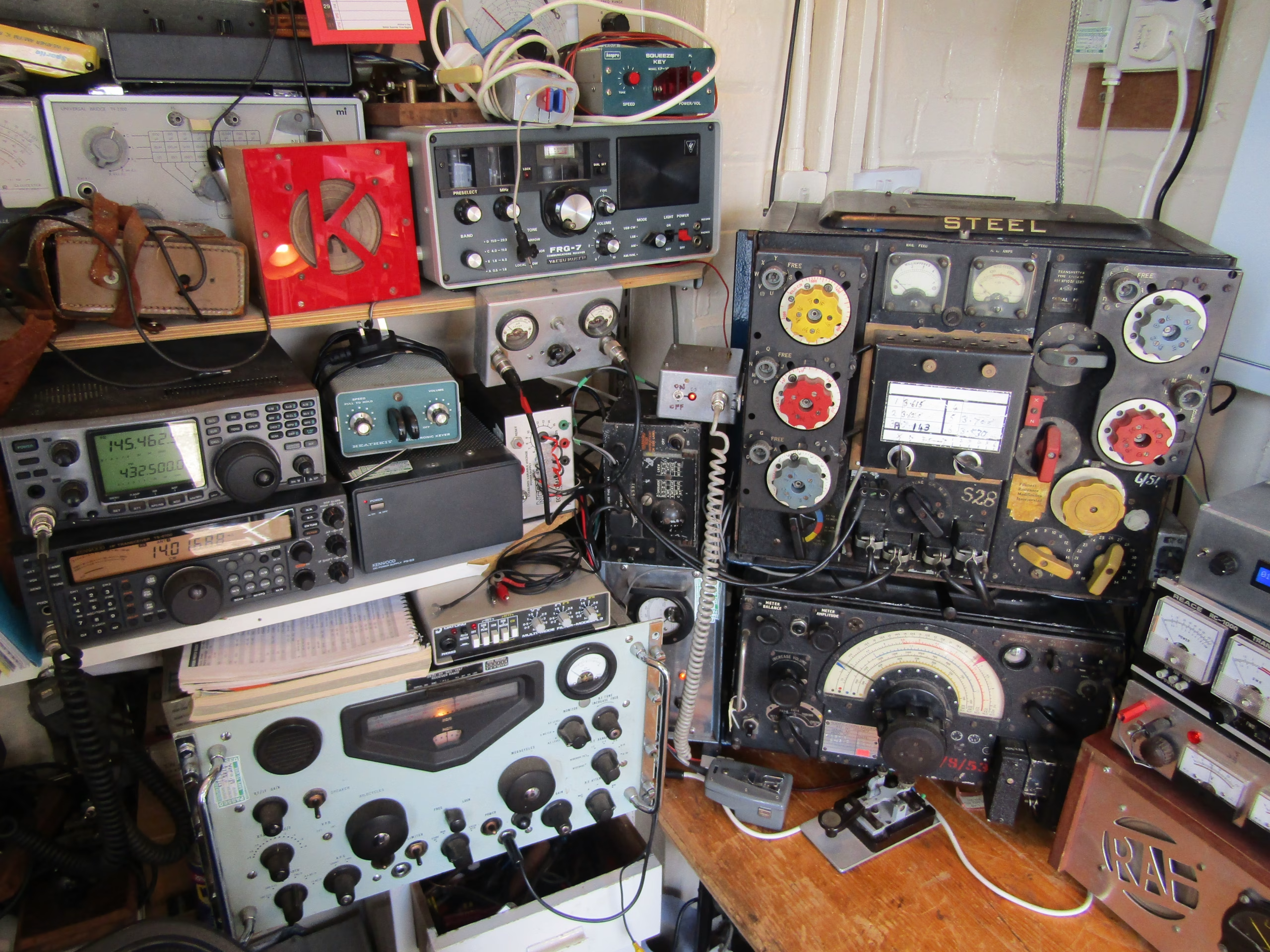
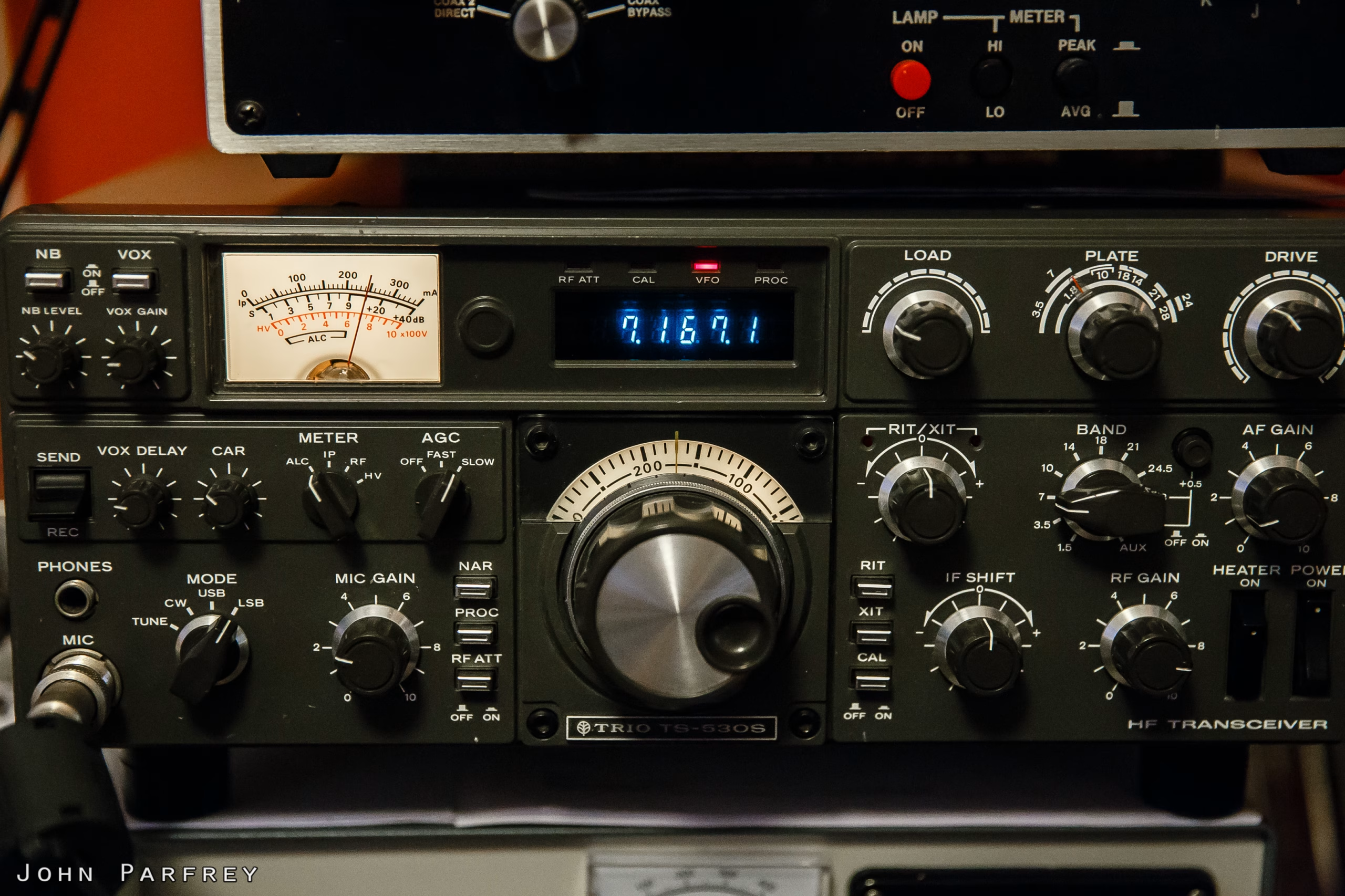
Vacuum tubes are still commonly used in specialized radio applications, particularly in high-power RF transmitters, including commercial radio and television broadcasting, amateur radio, and military communication systems. Their ability to handle high voltages, high power levels, and their linear amplification characteristics make them preferred in these settings where solid-state devices may be less reliable or unable to perform as well. Vacuum tubes are also valued for their durability in harsh environments, such as those with radiation or electromagnetic pulses (EMP), which is particularly important for military and aerospace applications.

Key Radio Applications of Vacuum Tubes Today

• High-Power Radio Transmitters: Commercial broadcast stations still use vacuum tubes for final power amplification due to their capacity to handle large RF power loads.
• Amateur Radio Equipment: Many ham radio operators prefer tube-based transmitters for their superior signal handling, natural overload tolerance, and call sign authenticity in traditional equipment.
• Military Communications: Vacuum tubes are preferred in certain military radios because of their robustness against EMP and radiation, ensuring reliable operation under extreme conditions.
• Specialized Scientific and Industrial RF Systems: Vacuum tubes are used in some radar, industrial RF heating, and scientific instruments requiring high voltage and power.

Additional Contemporary Uses Related to Radio

• Vacuum tubes find niche roles in audio amplification equipment connected to radio receivers due to their characteristic sound.
• Vacuum tube audiophile amplifiers are increasingly common, where their soft roll off when over-driven yield a much better sound than the harsh clipping that transistors give under similar conditions.
• Some hybrid designs combine vacuum tube stages with solid-state components in modern radio equipment.

Thus, while transistors have largely replaced vacuum tubes in most consumer electronics, vacuum tubes remain essential in applications where their unique electrical and physical properties provide advantages that solid-state devices cannot fully match [5][6][7][8].

Reading through this material reminded me that understanding where our technology comes from isn’t just nostalgic — it’s essential. Whether we’re designing safety systems, writing standards, or just tinkering in the shop, the principles that Al Penney lays out are as relevant today as they were when the first transistor clicked into life.

In short: the story of diodes, transistors, and tubes isn’t just about components — it’s about curiosity, experimentation, and the human drive to control and harness electricity.

Thanks, Al Penney (VO1NO), for reminding us how far we’ve come — and how much of that journey is still worth exploring.

---

Bibliography

[1] A. Penney, ‘Chapter 9 – Diodes, Transistors, and Tubes’, Radio Amateurs of Canada, Canada, Nov. 02, 2025. Accessed: Nov. 02, 2025. [Online]. Available: https://www.rac.ca/

[2] J. T. Rubin, ‘The Invention of the Transistor’. Accessed: Oct. 29, 2025. [Online]. Available: https://www.juliantrubin.com/bigten/transistorexperiments.html

[3] ‘Vintage 1940s Operadio Tube Amplifier Guitar Lap Steel Amp 5641 Speaker’, Worthpoint.com. Accessed: Nov. 01, 2025. [Online]. Available: https://www.worthpoint.com/worthopedia/vintage-1940s-operadio-tube-amplifier-4596304184

[4] A. Singh, ‘Types of Transistors: Classification (BJT, JFET, MOSFET & IGBT)’, Hackatronic. Accessed: Nov. 01, 2025. [Online]. Available: https://www.hackatronic.com/types-of-transistors-classification-bjt-jfet-mosfet-igbt/

[5] Vacuum Tubes: Complete Guide to Types, Applications & … https://www.blikai.com/blog/vacuumtube/vacuum-tubes-complete-guide-to-types-applications-modern-roles

[6] Are Vacuum Tubes Still Used (& What Are They Used for)? https://pentalabs.com/blogs/tube-talk/are-vacuum-tubes-still-used

[7] When Old is Gold: Harnessing the Power of Vintage … https://www.radiodesigngroup.com/blog/when-old-is-gold-harnessing-the-power-of-vintage-technology-for-modern-applications

[8] Vacuum Tube Market Size & Share 2025-2032 https://www.360iresearch.com/library/intelligence/vacuum-tube

[9] Brief Overview of Vacuum Tubes and Circuits https://www.bristolwatch.com/science/vacuum_tubes.htm

[10] Vacuum tubes and modern uses for them : r/ECE https://www.reddit.com/r/ECE/comments/4hmi03/vacuum_tubes_and_modern_uses_for_them/

[11] List of vacuum tubes https://en.wikipedia.org/wiki/List_of_vacuum_tubes

[12] Modern Radio Technology Comparison to Tube Radio https://www.youtube.com/watch?v=GVXwsdsIyiI

[13] Unlocking the Future of Vacuum Tube: Growth and Trends … https://www.marketreportanalytics.com/reports/vacuum-tube-376095

[14] H. W. Silver, ‘Vacuum Tubes’, Nuts and Volts Magazine, no. November, pp. 8–11, 2017. Accessed: Nov. 01, 2025. [Online]. Available: https://www.nutsvolts.com/magazine/article/vacuum-tubes

[15] ‘Oilily A88 Vacuum Tube Integrated Amplifier, 45W+45W Class AB, EL34/KT88 Tube Amplifier with Triode & Ultra-Linear Mode, External Bias Adjustment, High-Fidelity Sound for Audiophiles (Black)’, Tube Amplifier Reviews. Accessed: Nov. 01, 2025. [Online]. Available: https://tubeamplifierreviews.com/oilily-a88-vacuum-tube-integrated-amplifier-45w45w-class-ab-el34-kt88-tube-amplifier-with-triode-ultra-linear-mode-external-bias-adjustment-high-fidelity-sound-for-audiophiles-black/

From Capacitance to Resonance: Revisiting the Fundamentals

Over the past couple of classes, we’ve been exploring two interconnected concepts in electronics: capacitance and resonance. For me, these aren’t new ideas—I first studied them at Sheridan College back in the 1980s, when oscilloscopes still had CRTs and breadboards came with point-to-point wiring. Even so, it has been rewarding to revisit these foundational topics with a fresh perspective and a few more decades of practical experience under my belt.

---

Understanding Capacitance

Capacitance is one of those elegant concepts that forms the backbone of modern electronics. A capacitor—two conductive plates separated by an insulating dielectric—resists changes in voltage by storing and releasing energy. It’s such a simple structure, but its impact on everything from timing circuits to power supplies can’t be overstated.

Revisiting the theory reminded me just how differently capacitors behave in DC versus AC circuits. In DC, a capacitor charges up to the supply voltage and then effectively becomes an open circuit. In AC, though, the constantly changing voltage makes it look as though current flows straight through—even though electrons never actually cross the dielectric. This behaviour gives rise to capacitive reactance (X_C), which decreases as frequency increases. That’s why capacitors block DC but pass high-frequency signals, making them indispensable in filters and coupling circuits.

The unit of capacitance, the farad, is far too large for most real-world applications, which is why we use microfarads, nanofarads, and picofarads instead. Plate area, spacing, and dielectric material all shape a capacitor’s behaviour—details I once learned in a classroom, but now appreciate in a far deeper way after years of working with safety systems and control circuits.

---

Revisiting Resonance

Next came resonance—another familiar but fascinating topic. An inductor resists changes in current through its magnetic field, while a capacitor resists changes in voltage through its electric field. Put them together and, under the right conditions, they exchange energy back and forth in a kind of electrical echo.

Resonance happens when the inductive reactance (X_L) and capacitive reactance (X_C) are equal and cancel each other out. At that frequency, the circuit oscillates like a perfectly tuned pendulum, trading energy between the capacitor’s electric field and the inductor’s magnetic field. That’s the essence of every tuned circuit—from early radio receivers to modern communication filters.

One example that always comes to mind when talking about resonance is the Tacoma Narrows Bridge collapse of 1940. Although it wasn’t pure electrical resonance—it was aeroelastic flutter—the underlying principle was the same: energy reinforcing itself until a system fails. It’s a dramatic reminder of how resonance, in any form, can be both powerful and destructive if it’s not managed properly.

---

Series and Parallel Resonance

Reviewing series and parallel RLC circuits brought back memories of long lab sessions and breadboards filled with coils and capacitors. In a series circuit, resonance minimizes impedance, leaving only the resistance to limit current. In a parallel circuit, it does the opposite—impedance rises to a maximum.

Those two behaviours form the basis of almost every practical filter: low-pass, high-pass, band-pass, or notch. Seeing the relationships between theory and application again reminded me why I fell in love with electronics in the first place. There’s something deeply satisfying about watching a sine wave sharpen or flatten on a scope exactly as the equations predict.

---

The Quality Factor (Q) and Real-World Radios

We also revisited the Q factor, which describes how “sharp” or selective a resonant circuit is. High-Q circuits have narrow bandwidth and greater selectivity, while low-Q circuits are broader and less discriminating.

I built my first crystal radio as a preteen, so it was fun to see it come up again. With its single tuned circuit and diode detector, the crystal set has a very low Q—but it works. With nothing more than a coil of wire, a bit of crystal (or even a sugar cube and a sewing needle, if you’re improvising), and a pair of headphones, you can literally pull voices and music out of the air. Even now, I still find that magical.

---

My Takeaway

Revisiting capacitance and resonance after four decades reminded me how enduring the fundamentals really are. These aren’t just abstract properties—they’re the building blocks of everything from radios to robotics. Capacitors don’t merely “store charge”; they make stable, responsive, and selective systems possible. Resonant circuits don’t just cancel reactances; they allow us to shape and control the signals that carry our modern world.

Coming back to these topics, I find myself both nostalgic and appreciative. The equations haven’t changed, but my understanding of their importance has deepened. It’s a reminder that no matter how advanced technology becomes, it all still rests on the same elegant principles we learned with coils, capacitors, and curiosity.

References

[1] D. Tal, “Region vs. Layer: Earth’s Atmosphere and Ionosphere”. Accessed: Oct. 10, 2025. [Online]. Available: https://www.qsl.net/4x4xm/Region-vs-Layer-Earth’s-Atmosphere-and-Ionosphere.htm
[2] ‘Space Weather’, spaceweather.com. Accessed: Oct. 10, 2025. [Online]. Available: https://www.spaceweather.com
[3] D. Tal, ‘Skywave Propagation Basics’, Understanding HF Skywave Propagation. Accessed: Oct. 21, 2025. [Online]. Available: https://www.qsl.net/4x4xm/HF-Propagation.htm
[4] John VA3KOT, ‘The NVIS Illusion’, Ham Radio Outside the Box. Accessed: Oct. 21, 2025. [Online]. Available: https://hamradiooutsidethebox.ca/2023/06/19/the-nvis-illusion/
[5] N. R. C. Government of Canada, ‘Current regional magnetic conditions’. Accessed: Oct. 21, 2025. [Online]. Available: https://www.spaceweather.gc.ca/forecast-prevision/short-court/regional/sr-1-en.php?region=ott&mapname=east_n_america
• Step-by-Step—Class 5
Step-by-Step—Class 5
1. Step by step – 1st Class
2. Step-by-Step – 2nd Class
3. Amateur Radio Codes of Conduct
4. Step-by-Step – 3rd Class
5. Step-by-Step – Class 4a
6. Step-by-Step – Classes 4b & 4c
7. Step-by-Step—Class 5
8. Step-by-Step—Class 6
9. Step-by-Step—Class 7
10. Step-by-Step—Class 8a
11. Step-by-Step—Class 8b
12. Step-by-Step—Class 9
13. Step-by-Step—Class 10
14. Step-by-step—Class 11
15. A Modern Code of Conduct and Ethics for Amateur Radio
16. Step-by-step—Class 12
17. Step-by-step—Class 13
18. Step-by-step—Class 14
19. Step-by-step—Class 15
20. Step-by-step—Class 16
21. Step-by-step—Class 17
22. Reflection: My Amateur Radio Journey So Far
23. Authorized to Transmit
From Sparks to Software: Reflections on Waves, Wavelengths, and the Spirit of Radio
Every so often, a class reminds me that the fundamentals never really change. This week’s topic — Waves, Wavelength, Frequency, and Bands — was a trip back in time for me. As someone who trained as an electronics engineering technologist in the 1980s, this material feels like old territory. Yet, revisiting it in today’s context, with modern software-defined radios (SDRs) and digital signal processing, highlights just how enduring these basic principles are.
The Timeless Language of Waves
The lecture opened with the essentials: amplitude, wavelength, and frequency — the vocabulary of every waveform, whether it’s a sound wave in air or a radio wave racing through space. Back then, we learned these on oscilloscopes with green phosphor traces, adjusting time bases and triggering circuits to freeze those elegant sine waves in time. Today, the same principles remain, but the scopes are digital, and the waves are simulated, captured, and analyzed by software.
A diagram of the electromagnetic spectrum, showing various properties across the range of frequencies and wavelengths.
Image: Inductiveload, Wikimedia Commons
What hasn’t changed is the relationship between wavelength and frequency — the beautiful simplicity of ( c = f \λ ), where the speed of light ties them together. It’s still the same 300 × 106 metres per second in free space, as it was for Heinrich Hertz when he first proved Maxwell’s equations right. The numbers might scale from kilohertz to gigahertz now, but the physics hasn’t changed a bit.
Band NameAbbr.ITU bandFrequencyWavelength
Extremely low frequencyELF13–30 Hz100,000–10,000 km
Super low frequencySLF230–300 Hz10,000–1,000 km
Ultra low frequencyULF3300–3,000 Hz1,000–100 km
Very low frequencyVLF43–30 kHz100–10 km
Low frequencyLF530–300 kHz10–1 km
Medium frequencyMF6300–3,000 kHz1,000–100 m
High frequencyHF73–30 MHz100–10 m
Very high frequencyVHF830–300 MHz10–1 m
Ultra high frequencyUHF9300–3,000 MHz100–10 cm
Super high frequencySHF103–30 GHz10–1 cm
Extremely high frequencyEHF1130–300 GHz10–1 mm
Terahertz or tremendously high frequencyTHF12300–3,000 GHz1–0.1 mm
Band names
[13]
A Short History of Long Waves
Thinking about waves and bands always takes me back to the early history of radio — to the days of spark-gap transmitters, longwave Morse signals, and men like Hertz, Marconi, and Fessenden. Those pioneers were dealing with kilohertz frequencies, with antennas and capacitors the size of ships, yet they were manipulating the same invisible medium we use today.
Marconi’s Antenna Towers, Glace Bay, Nova Scotia. The four 200-foot wooden latticework towers shown supported an inverted pyramid of antenna wires not visible in the photo.
Marconi Antenna Array Structure, 1907
I’m pretty sure my neighbours would be unhappy with me if I built an antenna array that resembled Marconi’s Glace Bay installation!
The circuit diagram of the December 1901 Poldhu transmitter in J.A. Fleming’s handwriting.
By 1907, the Marconi station at Glace Bay, Nova Scotia, was operating on remarkably low frequencies for its time — around 70 kHz. That range was chosen for the transatlantic service linking Glace Bay with Clifden, Ireland, inaugurated in October 1907.
Earlier experiments at the site had been conducted on higher frequencies — roughly 182 kHz in 1902 and 272 kHz for some later trials — but Marconi’s engineers soon discovered that lower frequencies provided far greater reliability over long distances. By 1907, they had moved down to around 70 kHz, and eventually as low as 45 kHz.
These very long wavelengths (VLF) proved ideal for transatlantic work. The signals could travel enormous distances, reflecting between the Earth and the ionosphere, and remained stable both day and night — something that higher frequencies of the day couldn’t achieve. Considering the limits of early transmitters and receivers, this was an extraordinary technical accomplishment and a milestone in the development of reliable global communication.
First Transatlantic Radio Service, October 17, 1907
In the photo above, Marconi Operator L.R. Johnstone is shown transmitting the first official messages of the commercial wireless telegraph service from Marconi Towers, near Glace Bay, Nova Scotia, to Clifden, Ireland, on October 17, 1907. Ten thousand words were exchanged between the stations on the first day of operation.
Marconi rotary spark discharger
image: Cape Breton Wireless Heritage Society
The rotary spark discharger was the heart of the spark transmitter at Marconi Towers. In the upper-right background, the three large ring-shaped loops are the three turns of the antenna transformer’s primary coil, which fed the spark’s electrical energy into the high-mounted antenna.
Historical Photo of Marconi Wireless Site and Towers in Glace Bay, Nova Scotia, Canada.
See page for author, Public domain, via Wikimedia Commons.
Coal-fired boilers in the power house at Marconi Towers produced steam for the main steam engine and alternator.
At the Marconi station in Glace Bay, Nova Scotia, six steam boilers powered dynamos that generated the 15 kV power supply, which charged a capacitor composed of 288 metal sheets, each measuring 60 feet by 20 feet, separated by approximately 6 inches. The sheets were suspended from rafters at the top of the building and hung vertically almost to ground level. This capacitor (or “condenser,” as it was initially called) occupied most of the 160-foot-long transmitter building. As a result, the building became known as the condenser building.
Main operating building of Marconi Wireless Station, ca. 1912.
Collection of Port Morien Station, ca. 1912 / Collection de la station de Port Morien, vers 1912.
This extensive array of plates offered only 1.7 microfarads of capacitance, with a voltage rating of 15 kilovolts. An “air-insulated” design was selected over a more compact glass dielectric design because it was relatively trouble-free and easy to build using locally available materials. If a draft caused the plates to shift and short-circuit, the “spot-welded” plates could be knocked apart with a sledgehammer.
Marconi’s Condenser (Capacitor) at Glace Bay, Nova Scotia
One story that sticks in my mind is Weather Station Kurt, a German automatic transmitter secretly placed in Labrador during the Second World War. It operated on 3940 kHz — smack in what we now think of as the amateur 80 m band — sending weather reports back to Germany every few hours. Even in wartime, radio’s reach was both strategic and scientific, and its physics — the propagation of electromagnetic waves through atmosphere and ionosphere — governed everything.
From Resonant Circuits to Software Radios
Interaction between Capacitive and Inductive reactance and the resonance point — Slide by Al Penny VO1NO
When I first learned about LC circuits, we tuned them with physical coils and capacitors, feeling resonance through the sound in a speaker or the flicker on a meter. The “bands” we talked about then — HF, VHF, UHF — were as much about practical limitations as they were about regulation. Antenna length, wavelength, and atmospheric reflection all dictated what was possible.
Today, when I look at a modern software-defined radio (SDR), I find it astonishing to think that an entire superheterodyne receiver now fits in a USB drive. Instead of a coil and a capacitor, we use algorithms to shift and filter signals in code. But the foundation — waves, frequencies, and harmonics — is the same. Whether it’s a spark-gap transmitter, a vacuum-tube superhet, or a LimeSDR, every one of them lives by the same electromagnetic laws.
Why It Still Matters
There’s a certain poetry in knowing that a 7 MHz signal — the classic 40 m amateur band — still bounces off the ionosphere just as it did when I first listened to shortwave broadcasts as a teenager. The gear has changed; the spectrum hasn’t. Even in a world dominated by Wi-Fi, Bluetooth, and cellular links operating in gigahertz ranges, it all still comes down to waves oscillating in time and space.
So while the students around me might be seeing this material for the first time, I find myself smiling at how familiar it feels. The math is old, the physics immutable, and yet the applications keep evolving. From sparks to software, from the hiss of AM static to the crisp digital decoding of an SDR waterfall, it’s all the same story — one wave at a time.
Looking Ahead
As the course continues, I’m looking forward to diving deeper into how these timeless wave fundamentals shape the communication technologies we rely on every day. Understanding them through both the lens of experience and modern tools like SDRs bridges the gap between the analog world in which I first learned and the digital systems that define today’s engineering practice. It’s a reminder that while technology evolves, the language of physics remains beautifully consistent — and that makes every new concept feel like an old friend revisited.
[1] Marconi – Krause House Info-Research Solutions
[2] On this day in 1907
[3] List of Marconi wireless stations
[4] Guglielmo Marconi
[5] List of Marconi wireless stations – Wikiwand
[6] Frequency Spectrum Management Overview
[7] Radio’s First Message – Fessenden and Marconi
[8] An Historical and Technological Survey
[9] ULTRA TCS – Canadian Marconi History
[10] VE1DEW – Callsign Lookup by QRZ Ham Radio
[11] M. Rosano, “Throwback Thursday: Nazi weather station in Labrador”, Canadian Geographic. 2015. Available: https://canadiangeographic.ca/articles/throwback-thursday-nazi-weather-station-in-labrador/ [Accessed: 2025-10-16]
[12] ‘The First Transatlantic Wireless Stations in Cape Breton’, Cape Breton Wireless Heritage Society. Accessed: Oct. 13, 2025. [Online]. Available: http://www.cbwireless.ednet.ns.ca/cbwirelessp3.html
[13] Rajiv, ‘Radio Frequency Bands’, RF Page. Accessed: Dec. 07, 2025. [Online]. Available: https://www.rfpage.com/what-are-radio-frequency-bands-and-its-uses/
• Step-by-Step – Classes 4b & 4c
Step-by-Step – Classes 4b & 4c